Chapter 4
Testing the generalization of the potential height framework
Abstract. Tropical cyclones (TCs) generate extreme storm surges that pose a significant and growing threat to coastal communities, a risk amplified by climate change. Identifying worst-case surge scenarios is computationally prohibitive using traditional simulation methods. This Chapter builds upon the new Bayesian optimization (BO) framework designed to efficiently discover TC trajectories that produce maximum storm surge heights from Chapter 3, known as the potential height. We present results from applying this framework to three distinct US coastal locations (New Orleans, Galveston, and Miami), demonstrating its ability to identify physically consistent worst-case scenarios under current and future climate conditions (calculated using the potential intensity and PI potential size from Chapter 2). Furthermore, we conduct sensitivity analysis of Gaussian Process (GP) kernel choices, a critical component of the BO surrogate model, which shows that the Matérn kernel chosen in Chapter 3 provides skillful predictions. Our findings broadly indicate that the choices made in Chapter 3 are sensible, that the random error in the BO results is relatively small, and that the BO framework generalizes reasonably well geographically.
4.1 Introduction
Tropical cyclones (TCs) are a primary driver of catastrophic storm surges, which can lead to extensive flooding and devastation in coastal regions (Resio and Westerink 2008). In a warming climate, the characteristics of TCs are changing (see e.g. Chapter 2), with projections indicating increases in average intensity, rainfall rates, and the proportion of the most severe storms (Knutson et al. 2020; GFDL 2024). Coupled with sea-level rise, these changes amplify the threat of coastal inundation, making the accurate assessment of potential storm surge heights a critical task for disaster preparedness and infrastructure planning (Oppenheimer et al. 2019).
An interesting challenge in hazard assessment is identifying the worst-case storm surge for a given location. This requires both considering the practical thermodynamic limits on TCs, and exploring a high-dimensional parameter space of how the TC characteristics, including track, intensity, size, and forward speed will interact with the complex geometry at the coast. High-fidelity hydrodynamic models like ADCIRC (Luettich et al. 1992) can numerically simulate surge events, but their computational expense makes a brute-force exploration of this parameter space intractable (Toro et al. 2008).
To address this challenge, Thomas et al. (2025, Chapter 3) introduced a framework for finding the potential height of storm surges using Bayesian optimization (BO), a sample-efficient global optimization technique for expensive black-box functions (see e.g. Shahriari et al. 2015; Brochu et al. 2010), while assuming the TC potential intensity and PI potential size produced through thermodynamic arguments (see Chapter 2). This framework not only provides a robust estimate of the upper bound on surge height but also improves the estimation of high-return-period events (e.g., 1-in-100 or 1-in-500 year events). The BO approach iteratively builds a probabilistic surrogate model of the surge response and uses an acquisition function to intelligently select the next set of TC parameters to numerically simulate, efficiently converging on the most impactful storm scenarios (see Ide et al. 2024 for contemporaneous work not using thermodynamic TC bounds).
This Chapter presents key results from this framework and investigates the sensitivity of its machine learning components, and a demonstration that it can generalize geographically. In Section Section 4.2.1, we detail the BO methodology and define the metrics of interest. In Section Section 4.3, we showcase its application to New Orleans, Galveston, and Miami and present a comparative analysis of Gaussian Process kernels for modeling the surge response. Finally, in Section Section 4.4, we outline critical areas for future work to refine and extend this approach.
4.2 Methods
4.2.1 A Bayesian Optimization Framework for Storm Surges
Our methodology treats the high-fidelity ADCIRC storm surge model (Luettich et al. 1992) as an expensive black-box function whose inputs are the parameters of an idealized TC. The goal of the BO algorithm is to find the input parameters that maximize the peak storm surge at a specified observation point, which is the closest point on the mesh to a city of interest (New Orleans, Miami, or Galveston).
The TC parameters we vary, \(x\), define a three-dimensional search space (see Table 3.2 for a summary of all framework parameters): the landfall point relative to the observation location, \(c \in \left(-2^{\circ}, 2^{\circ}\right)\); the bearing of approach, \(\chi\), constrained to approach from the ocean1; and the translation speed, \(V_t \in \left(0,\; 15 \right) \text{ m s}^{-1}\). The TC’s wind and pressure profiles follow the model of Chavas et al. (2015), with intensity and size fixed at their potential limits for the given climate conditions (see Section Section 4.2.3).
As in Chapter 3, the BO process begins by initializing a dataset with 25 points selected via Latin hypercube sampling (McKay et al. 1979) to ensure good initial coverage of the parameter space. Subsequent points are chosen sequentially by maximizing an acquisition function. We use the ADCIRC model (Luettich et al. 1992) to numerically simulate the storm surge for the observed point, and assume that the maximum sea surface height at the observed point has a small Gaussian noise \(\sigma_{\varepsilon}\), and define \(f(x)\) as the negative of the maximum storm surge height at that point during the simulation. Since standard BO libraries are formulated as minimisation problems, we negate the surge height so that minimising \(f\) is equivalent to maximising the storm surge. The problem setup is currently as follows:
\[\begin{align} &\text{\textbf{Objective:}}\quad x^{i}=\arg\min_{x\in\mathcal{X}\subset\mathbb{R}^{d}} f(x), \qquad f:\mathcal{X}\!\to\!\mathbb{R}\;\text{deterministic}. \\& \text{\textbf{Prior on }}f:\quad \hat{f} \sim \mathcal{GP}\!\bigl(0,k_{\mathrm{M52}}\bigr)\\& k_{\mathrm{M52}}(x,x') =\sigma_f^{2}\!\Bigl(1+\tfrac{\sqrt5 r}{\ell} +\tfrac{5r^{2}}{3\ell^{2}}\Bigr) \exp\!\Bigl(-\tfrac{\sqrt5 r}{\ell}\Bigr),\; r=\lVert x-x'\rVert_2. \\& \text{\textbf{Data (noisy):}}\quad \mathcal{D}_n=\{(x_i,y_i)\}_{i=1}^{n},\quad y_i = f(x_i) + \varepsilon_i,\; \varepsilon_i\sim\mathcal{N}(0,\sigma_\varepsilon^{2}). \\& \text{\textbf{Posterior surrogate:}}\quad \hat{f} \mid \mathcal{D}_n \sim \mathcal{GP}\!\bigl(\mu_n(\cdot),k_n(\cdot,\cdot)\bigr) \\& \text{\textbf{Acquisition (Max-Value Entropy Search):}}\notag\\& \alpha_{\mathrm{MES}}(x)= H\!\bigl[\hat{f}^{i}\mid\mathcal{D}_n\bigr] \;-\; \mathbb{E}_{\,y(x)\mid\mathcal{D}_n}\! \Bigl[ H\!\bigl[\hat{f}^{i}\mid \mathcal{D}_n\cup\{(x,y(x))\}\bigr] \Bigr],\\& \hat{f}^{i}=\min_{x\in\mathcal{X}}\hat{f}(x),\quad x_{n+1}=\arg\max_{x\in\mathcal{X}}\alpha_{\mathrm{MES}}(x). \end{align}\](4.1)
Here \(\mathcal{X}\subset\mathbb{R}^{d}\) is the bounded search space and \(f:\mathcal{X}\!\to\!\mathbb{R}\) is the objective we want to minimize. The random field \(\hat{f}\mid\mathcal{D}_{n}\sim\mathcal{GP}(\mu_{n},k_{n})\) is the posterior surrogate model; its mean \(\mu_{n}(x)\) is a point predictor, while the covariance \(k_{n}(x,x')\) (specified here by the Matérn-5/2 kernel \(k_{\mathrm{M52}}\) with signal variance \(\sigma_{f}^{2}\), length-scale \(\ell\) and pairwise distance \(r=\lVert x-x'\rVert_{2}\)) encodes remaining uncertainty. The data set \(\mathcal{D}_{n}=\{(x_{i},y_{i})\}_{i=1}^{n}\) contains the evaluations \(y_{i}=f(x_{i})\), assumed to have a small random noise. For any sample path of the GP, \(\hat{f}^{i}=\min_{x\in\mathcal{X}}\hat{f}(x)\) is its (global) minimum value; thus \(\hat{f}^{i}\) is a random variable. The Max-Value Entropy Search acquisition \(\alpha_{\mathrm{MES}}(x)\) measures the expected information gain about \(\hat{f}^{i}\) obtained by evaluating \(f\) at \(x\); the next experimental design point is \(x_{n+1}=\arg\max_{x}\alpha_{\mathrm{MES}}(x)\).
4.2.2 Metrics
We evaluate the performance of the BO framework using two main categories of metrics: convergence to the optimal surge height and predictive accuracy of the GP surrogate model.
- Convergence to the Optimal Surge Height
-
We track the maximum surge height found as a function of the number of ADCIRC simulations. This metric assesses how quickly the BO algorithm converges to the worst-case scenario.
- Robustness Across Random Seeds
-
To ensure the reliability of the BO results, we repeat each experiment with multiple random seeds and report the mean and standard deviation of the maximum surge heights found.
- Approximate Simple Regret
-
The approximate simple regret, \(r_i\), quantifies the suboptimality of the best point found after \(i\) iterations. It is defined as the difference between the function value of the best recommendation so far, \(x_n^{\text{best}}\), and the true minimum function value, \(f(x^*)\), (estimated by the lowest value found over all experiments), \[\begin{equation} r_n = f(x_i^{\text{best}}) - f(x^*), \end{equation}\](4.2) where \(x_n^{\text{best}} = \arg\min_{x_i \in \{x_1,\; \dots,\; x_n\}} y_i\). This quantifies the efficiency of the optimization process, and a lower simple regret indicates a more efficient optimization process.
- Predictive Accuracy of the GP Surrogate
-
We assess the surrogate model’s accuracy against a test set, which evaluates how well the GP captures the underlying function.
- Coefficient of determination (\(r^2\))
-
The \(r^2\) score indicates the proportion of the variance in the true surge heights that is predictable from the GP model. An \(r^2\) of 1 indicates a perfect fit. \[\begin{equation} r^2 = 1 - \frac{\sum_{i=1}^{N_{\text{test}}} (y_i - \mu_n(x_i))^2}{\sum_{i=1}^{N_{\text{test}}} (y_i - \bar{y})^2} \end{equation}\](4.3) where \(\bar{y} = \frac{1}{N_{\text{test}}} \sum_{i=1}^{N_{\text{test}}} y_i\) is the mean of the true surge heights in the test set.
- Root Mean Square Error (RMSE)
-
The RMSE measures the standard deviation of the prediction errors, providing a measure of the surrogate’s overall predictive performance in the units of the target variable (meters), where an RMSE of 0 indicates a perfect fit. It is defined as, \[\begin{equation} \text{RMSE} = \sqrt{\frac{1}{N_{\text{test}}} \sum_{i=1}^{N_{\text{test}}} (y_i - \mu_n(x_i))^2}, \end{equation}\](4.4) where \(y_i\) is the true surge height for the \(i\)-th test point, and \(\mu_n(x_i)\) is the posterior mean prediction from the GP for the \(i\)-th test point.
- Mean Predictive Log-Likelihood
-
The mean predictive log-likelihood of the model on the test set is evaluated, given the model parameters, so that we can assess how well the model fits probabilistically. For a single point, the predictive log-likelihood is defined as, \[\begin{equation} \mathcal{L}_i= \log p\!\bigl(y_i \mid x_i,\mathcal{D}_n\bigr) =-\tfrac12\Bigl[ \log\!\bigl(2\pi\bigl(\sigma_n^{2}(x_i)+\sigma_{\text{obs}}^{2}\bigr)\bigr) + \frac{\bigl(y_i-\mu_n(x_i)\bigr)^2} {\sigma_n^{2}(x_i)+\sigma_{\text{obs}}^{2}} \Bigr]. \end{equation}\](4.5) where \(\sigma_n^2(x_i)\) is the variance of the GP surrogate model at \(x_i\), \(\sigma_{\text{obs}}^2\) is the fitted observation noise, and \(\mu_n\) is the mean of the model at the test point. The predictive log-likelihood is a measure of how well the model fits the data, with higher values indicating a better fit. We then average over all test points to get the final score, \(\bar{\mathcal{L}}\).
4.2.3 Potential Intensity and Size for US Coastal Cities
We choose three coastal cities in the United States with distinct geographic and climatic characteristics: New Orleans, Louisiana; Galveston, Texas; and Miami, Florida. These locations are selected to represent a range of coastal environments, from the semi-enclosed basin of New Orleans to the open coastlines of Galveston and Miami. Each city has an infamous history of significant storm surge events, making them ideal candidates for testing the BO framework. We use the same ADCIRC mesh as in Chapter 3, with a resolution of approximately 1 km near the coast and a coarser resolution offshore. As this mesh covers all three locations, we reuse it in each case. The mesh includes detailed bathymetry and topography data to accurately capture the coastal geometry and its influence on storm surge dynamics.
The potential intensity (PI), \(V_p\) and the PI potential size (PS) that is possible at that intensity2 of TCs for each location are calculated using the methods outlined in Chapter 2. For the 2015 and 2100 climate conditions, we used the r4i1p1f1 member of CESM2 model from the SSP5-8.5 scenario, taking data from the August monthly average, selected at the closest ocean grid point to each city after the data had been bilinearly regridded to a 0.5\(^{\circ}\) grid using CDO. The PI and PS values for each location and time period are summarized in Table 4.1. As is expected, the effect of global warming (as indicated by the increasing sea surface temperature) leads to an increasing potential intensity and potential size.
| Location | Year | SST [\(^{\circ}\)C] | PI \(V_p\) [m s\(^{-1}\)] | \(r_3\) [km] | \(r_{a3}\) [km] |
|---|---|---|---|---|---|
| New Orleans | 2015 | 31.3 | 105.0 | 24.4 | 1500 |
| 2100 | 34.8 | 111.4 | 28.4 | 1743 | |
| \(\Delta\) | 0.9% | 6.1% | 16% | 16% | |
| Galveston | 2015 | 30.5 | 94.9 | 29.8 | 1590 |
| 2100 | 34.3 | 105.0 | 31.9 | 1811 | |
| \(\Delta\) | 1.3% | 10.6% | 7% | 14% | |
| Miami | 2015 | 30.4 | 96.8 | 31.5 | 1727 |
| 2100 | 33.5 | 99.5 | 36.0 | 1928 | |
| \(\Delta\) | 1.0% | 2.7% | 14% | 12% |
4.3 Results
4.3.1 Application to US Coastal Cities
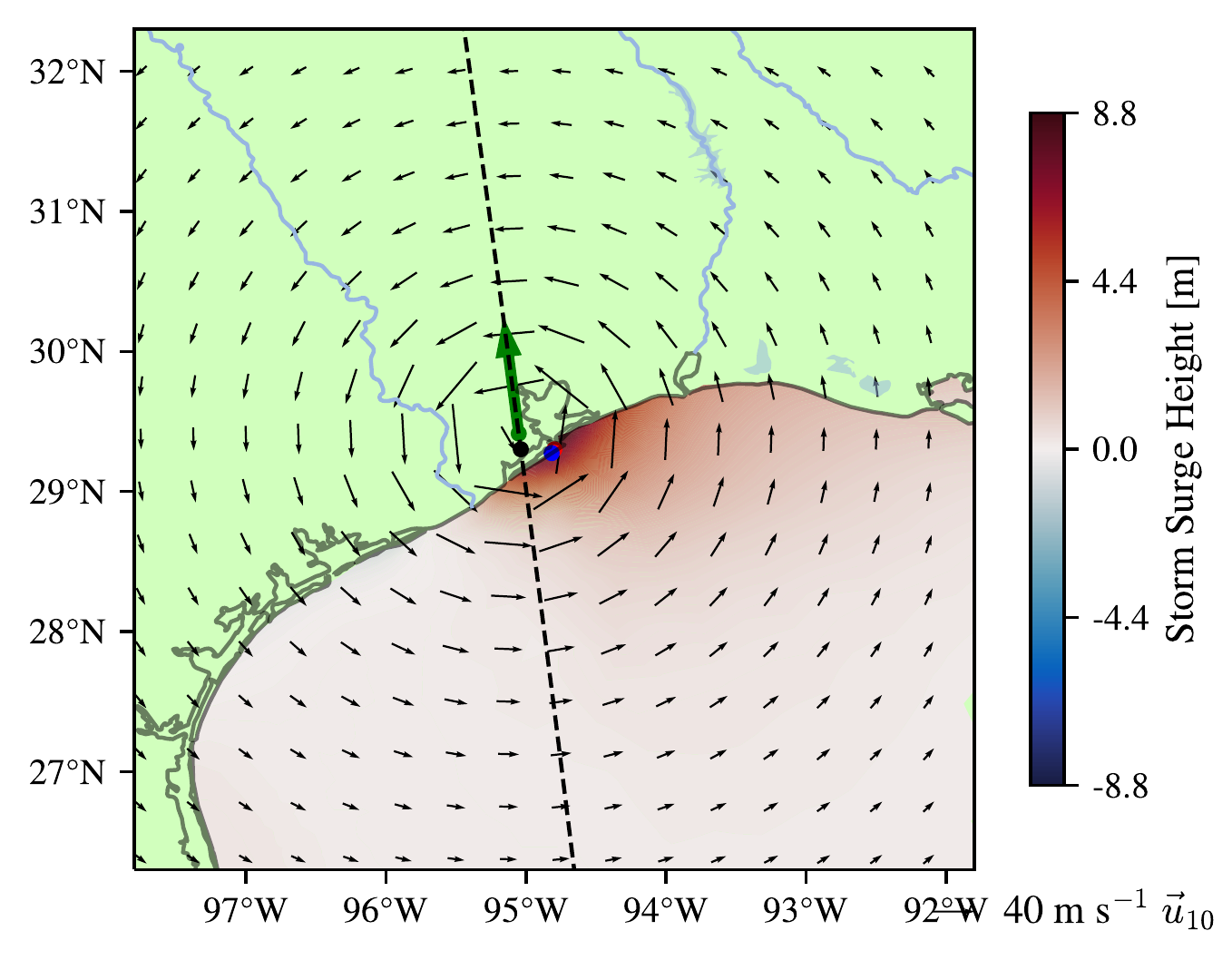
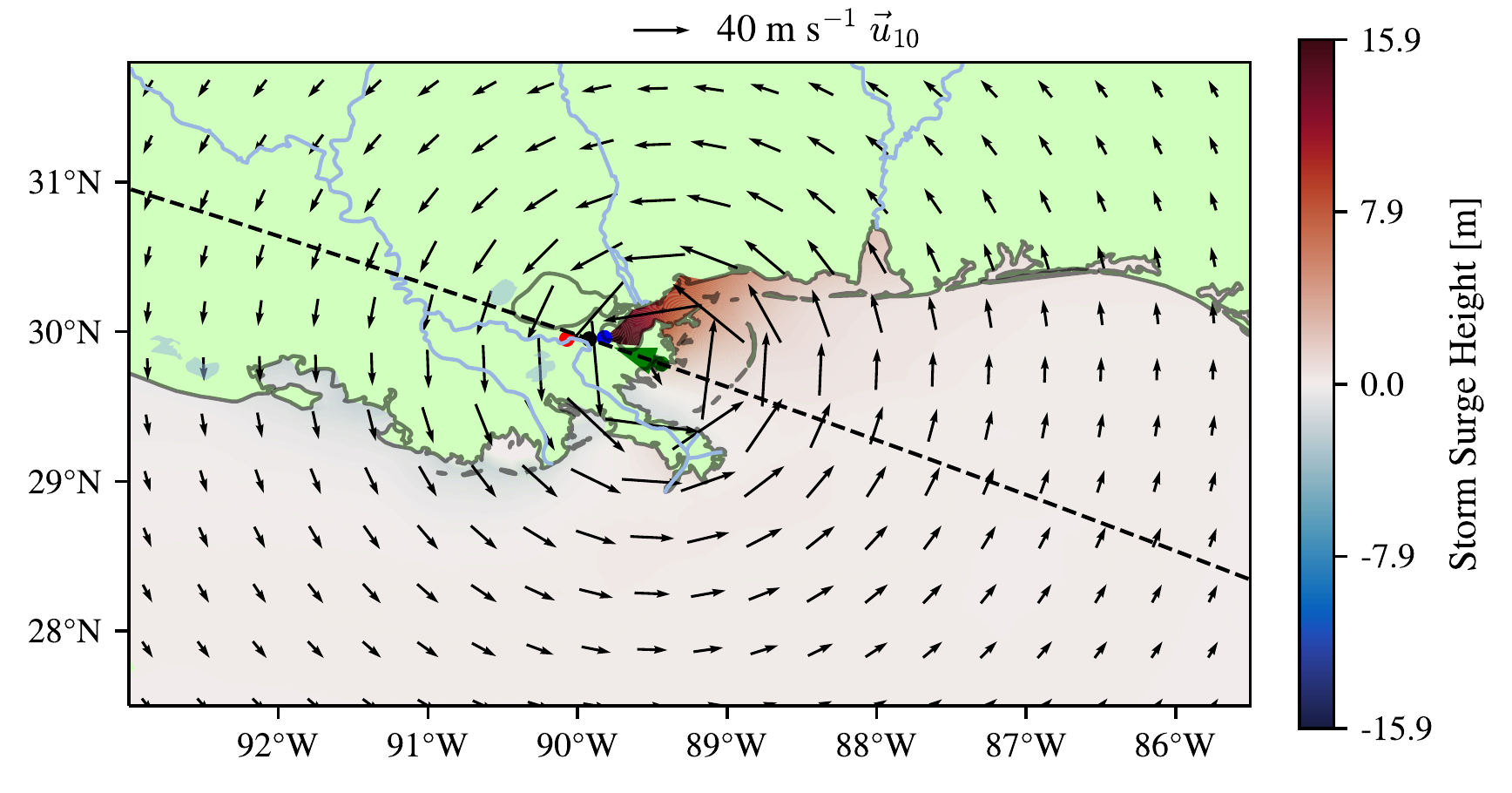
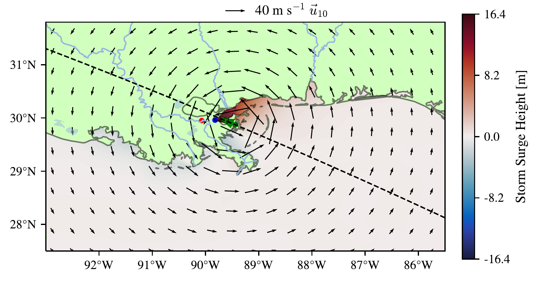
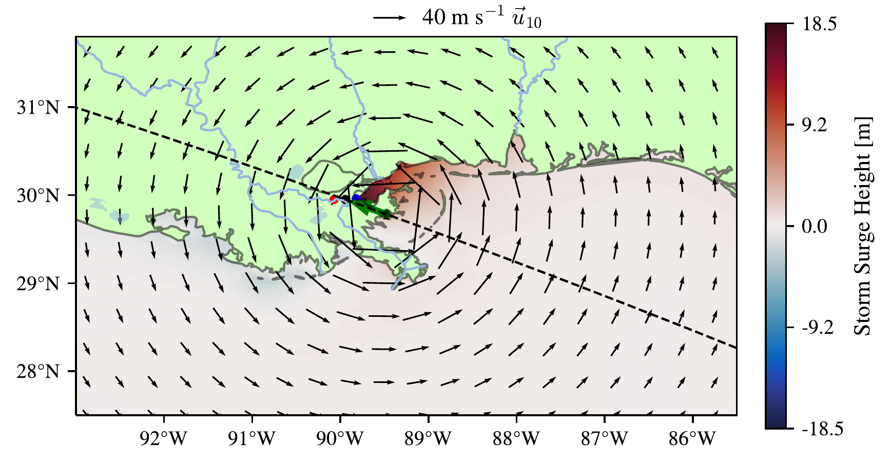
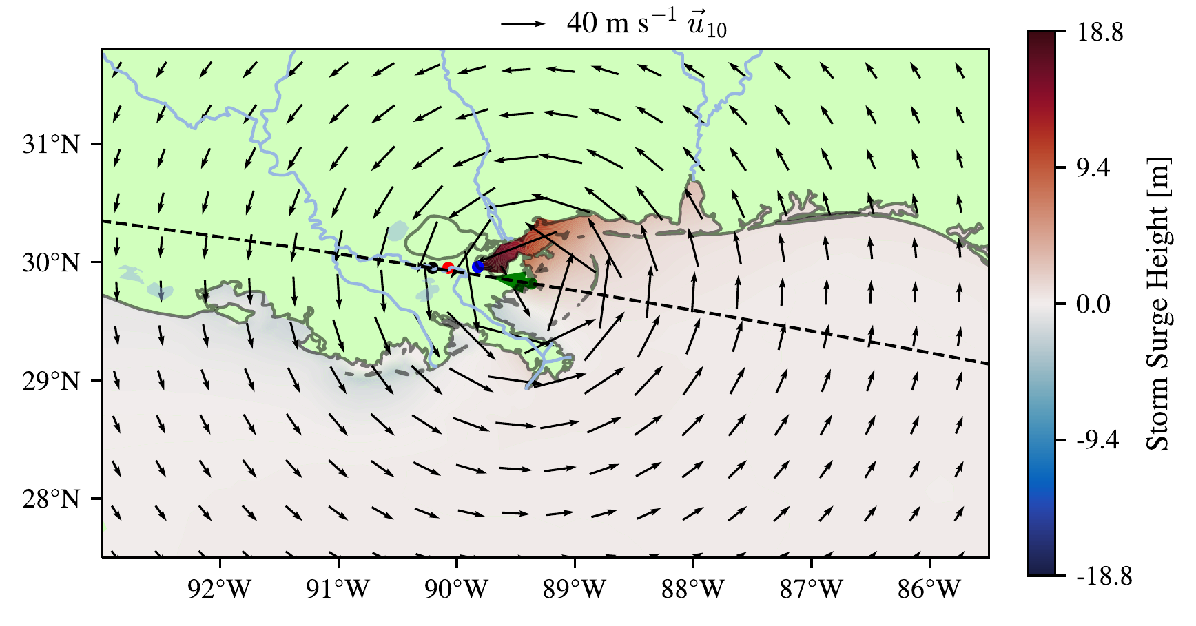
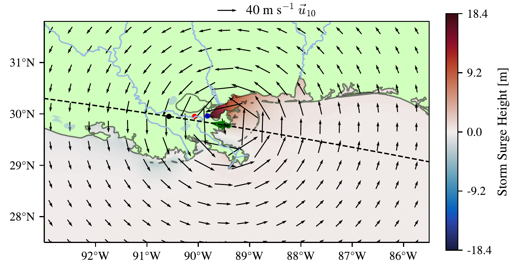
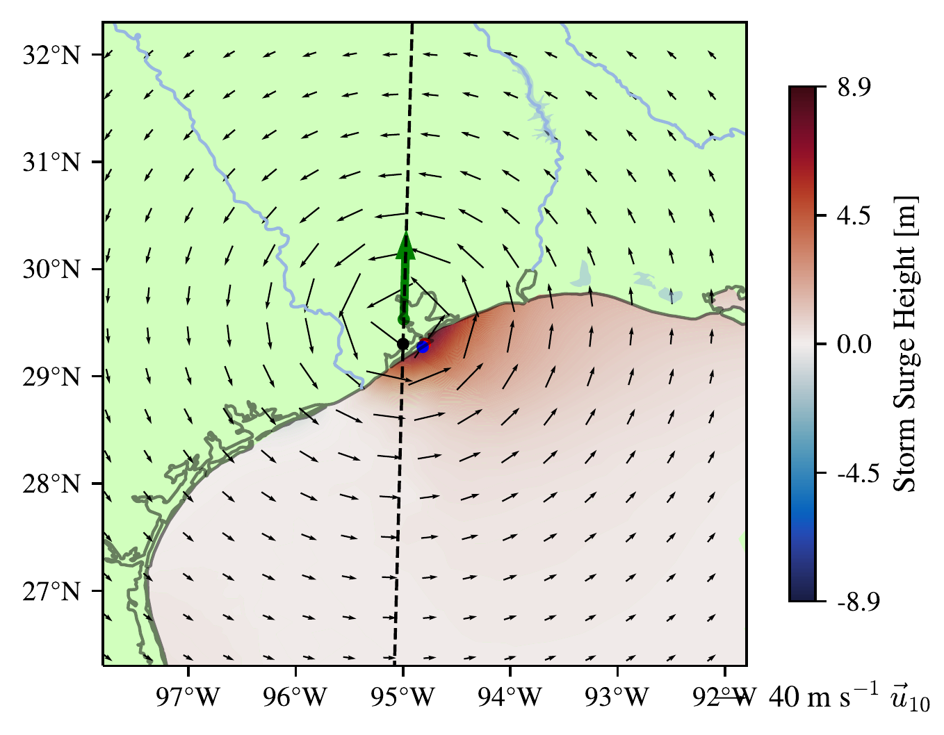
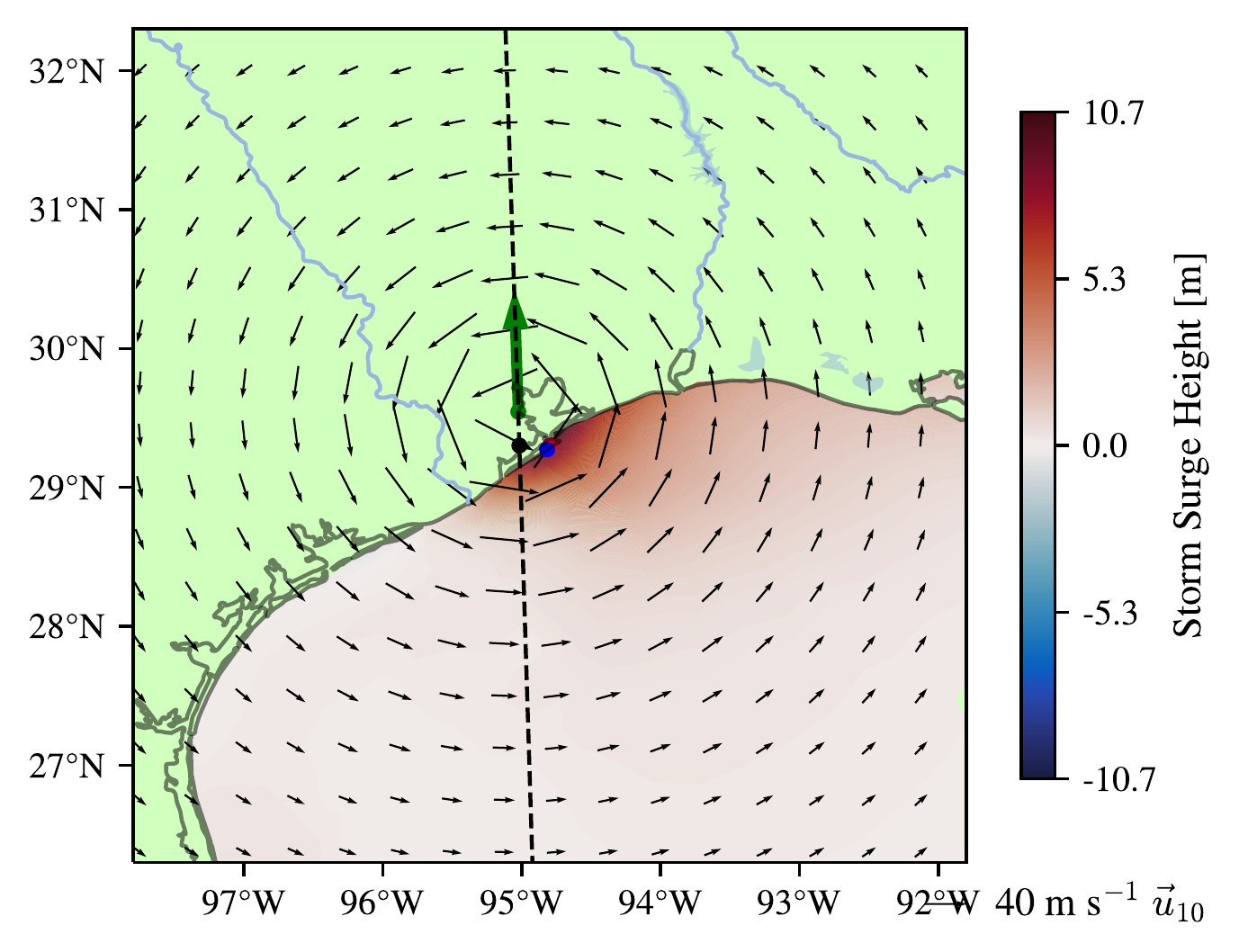
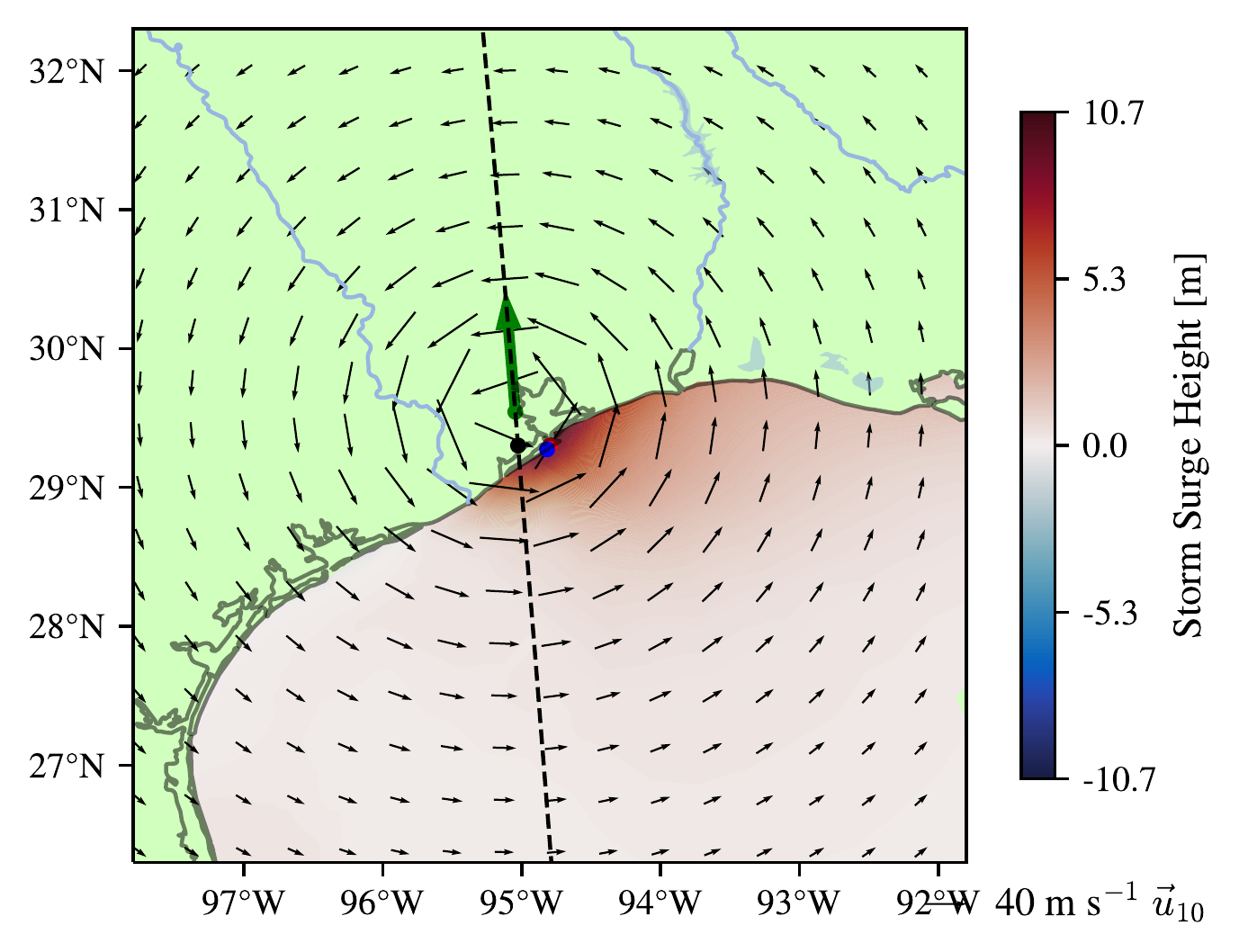
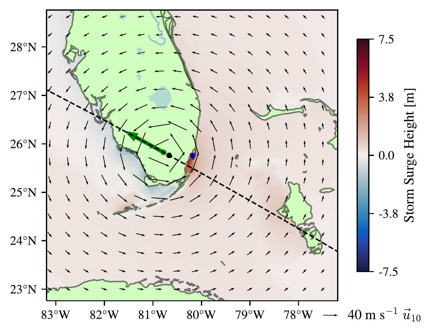
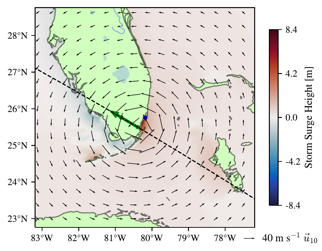
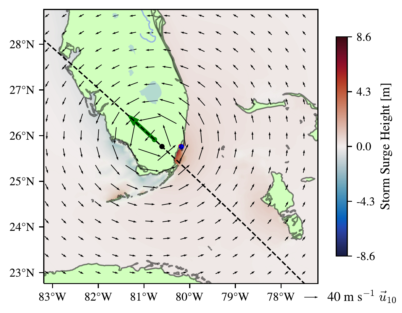
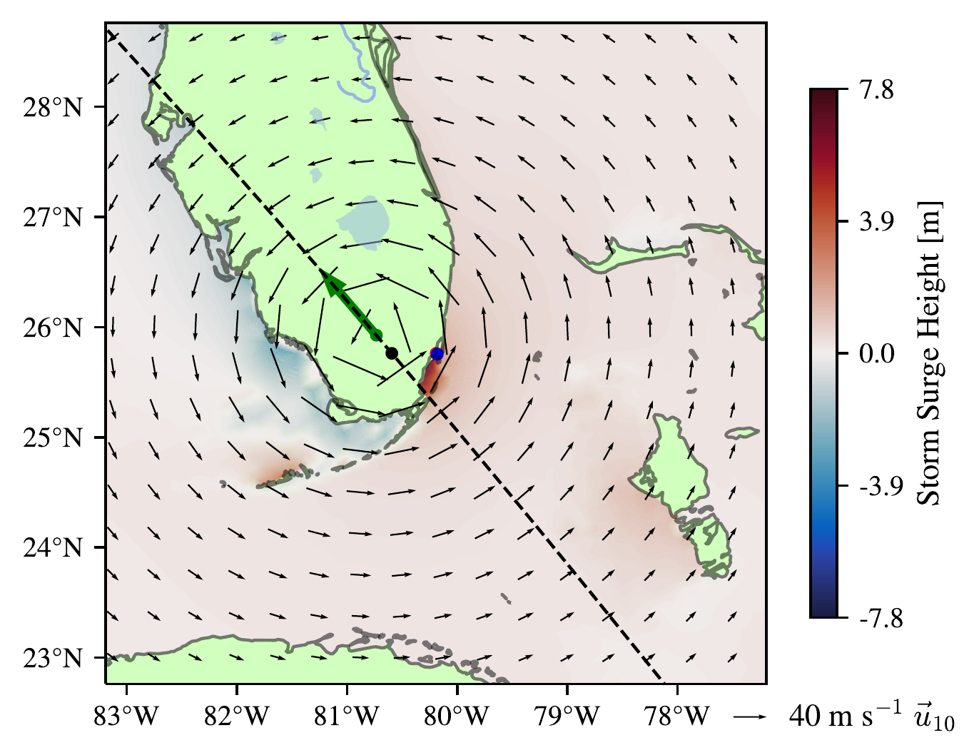
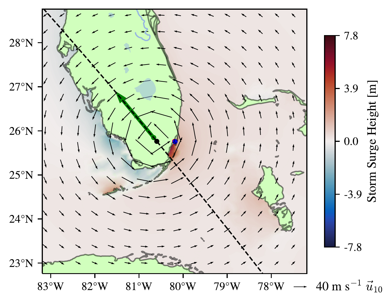
We first present a summary of the results of applying the BO framework to find the worst-case storm surges for New Orleans, Galveston, and Miami using TC potential intensity and size for August 2015 climate conditions (with a summary of the same procedure applied to 2100 in Table 4.2). The results, shown in Figures 4.2, 4.3, and 4.4, reveal distinct optimal TC trajectories tailored to each local geography. They are shown at the moment of maximum storm surge height for the observation point, i.e. a snapshot of the numerical simulation at which the potential height found is realized. The dashed black line on each shows the straight line trajectory of the TC, the green arrow shows the direction of travel, and its size is proportional to the translation speed. The blue dot is the observation point, the red dot is the city itself, and the black dot is the “impact point" which is the point at which the TC goes through at a constant time in each numerical simulation. The colormap shows the storm surge height, and the black quivers show the 10m wind vectors.
For New Orleans (Figure 4.2), located within a semi-enclosed bay system, the worst-case surge of 15.8 m is produced by a very slow-moving TC (\(V_t=1.23 \text{ m s}^{-1}\)). This slow speed allows the cyclonic winds to efficiently pile water into the bay. In contrast, for Galveston and Miami (Figures 4.3 and 4.4), which are on open coastlines, the optimal trajectories involve much faster translation speeds (\(V_t=13.9 \text{ m s}^{-1}\) and \(V_t=13.1 \text{ m s}^{-1}\), respectively). This is consistent with previous findings that faster-moving storms tend to produce higher surges on open coasts (Lockwood et al. 2022). In all cases, the optimal track positions the northeast quadrant of the storm, typically the region of strongest winds and surge generation, travelling over the observation point.
Repeating the experiments under a high-emissions 2100 climate scenario (SSP5-8.5) consistently yields higher potential heights (Table 4.2), highlighting the framework’s utility for climate change impact assessment. It is interesting to note that Galveston’s largest relative potential height increase of 21.7% corresponds to a 10.6% increase in potential intensity and a 14% increase in PI potential outer size (Table 4.1). Whereas, Miami’s much smaller relative potential height increase of 7.1% corresponds to a lower potential intensity increase of 2.7% and a lower PI potential outer size increase of 12%. New Orleans, with its very high storm surge sensitivity (caused both by the bay and the large area of shallow water around it) has the largest absolute increase in potential height of 2.4 m, but an intermediate relative potential increase of 15.1% corresponding to its intermediate potential intensity increase of 6.1% and PI potential outer size increase of 16%. Notably, the optimal trajectories are broadly unchanged between 2015 and 2100: only the surge magnitude increases while the track parameters remain similar. This suggests that the basic geometry of the coastline, rather than the intensity or size of the storm, is the primary determinant of the worst-case trajectory. If the assumptions of a fixed coastline and sea level were relaxed to include sea-level rise and coastal evolution, the optimal trajectory could differ between the two periods.
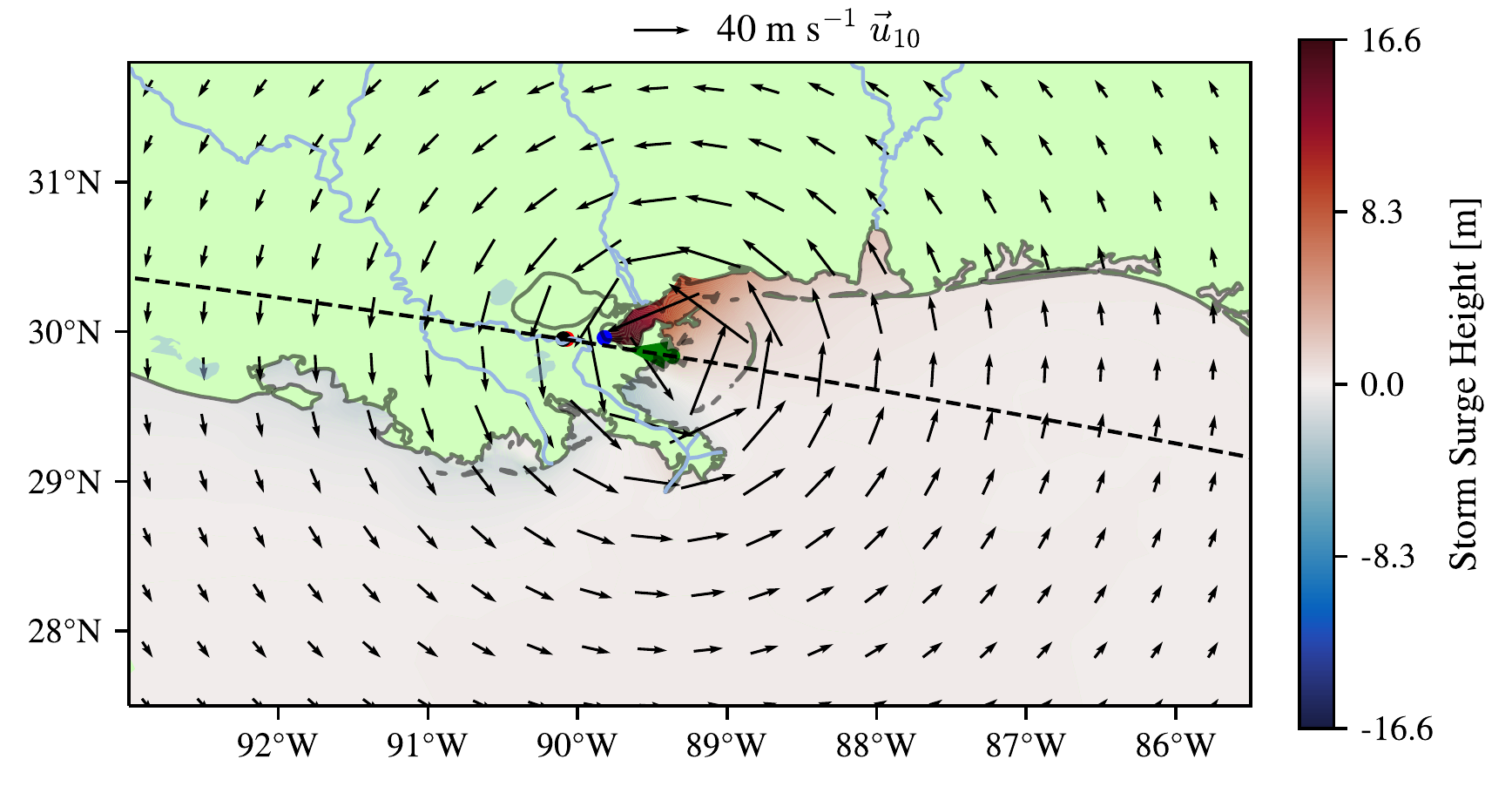
\(V_t=13.9\text{ m s}^{-1}\), \(\chi=-6.55\;^{\circ}\), \(c=-0.24\;^{\circ}\)E.
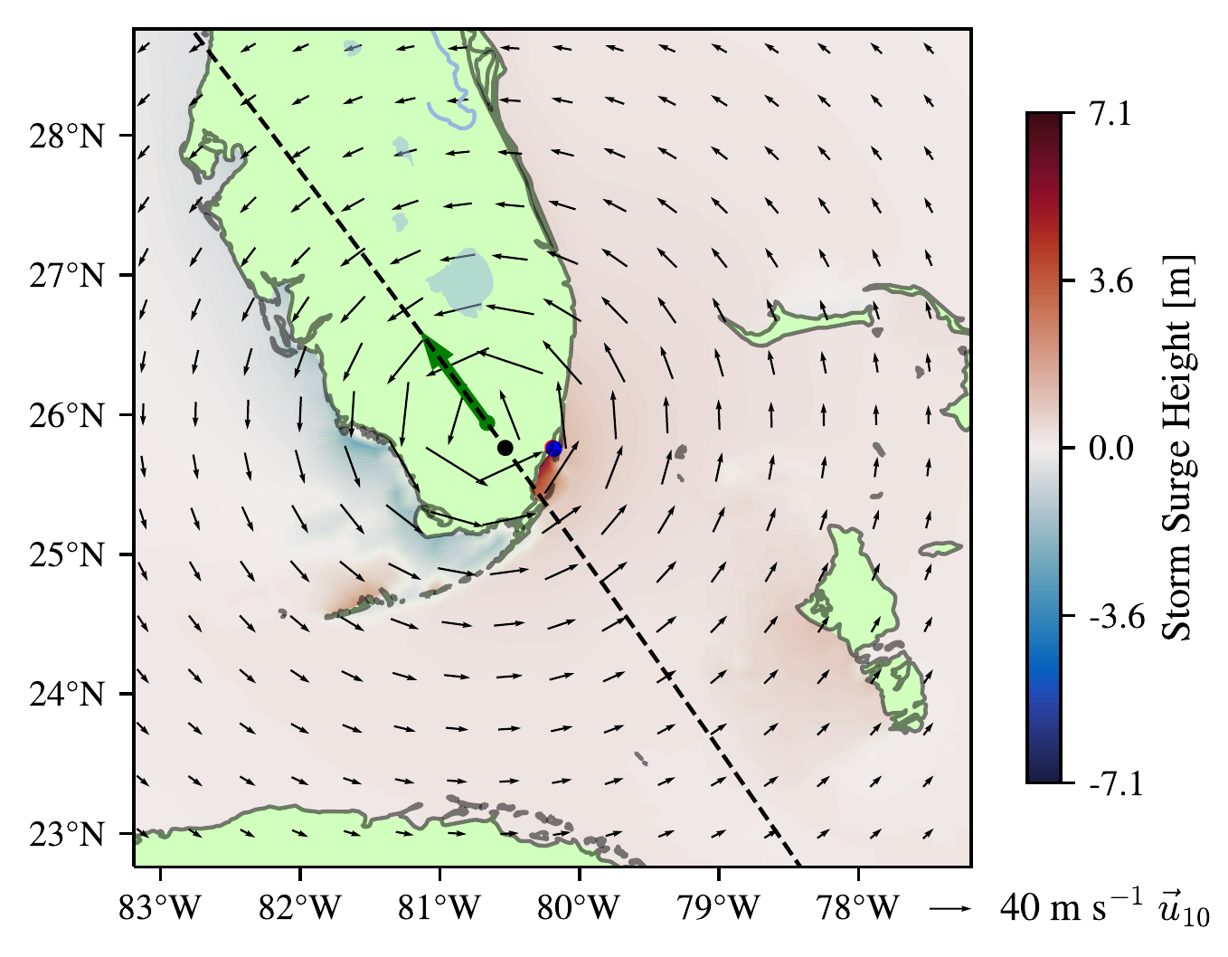
\(V_t=13.1 \text{ m s}^{-1}\), \(\chi=-33.3\;^{\circ}\), \(c=-0.34\;^{\circ}\)E.
| Location | 2015 | 2100 | \(\boldsymbol{\Delta}\) |
|---|---|---|---|
| New Orleans | 15.8 m | 18.2 m | 2.4 m (15.1%) |
| Galveston | 7.8 m | 9.5 m | 1.7 m (21.7%) |
| Miami | 5.6 m | 6.0 m | 0.4 m (7.1%) |
4.3.2 Investigating random error in solution
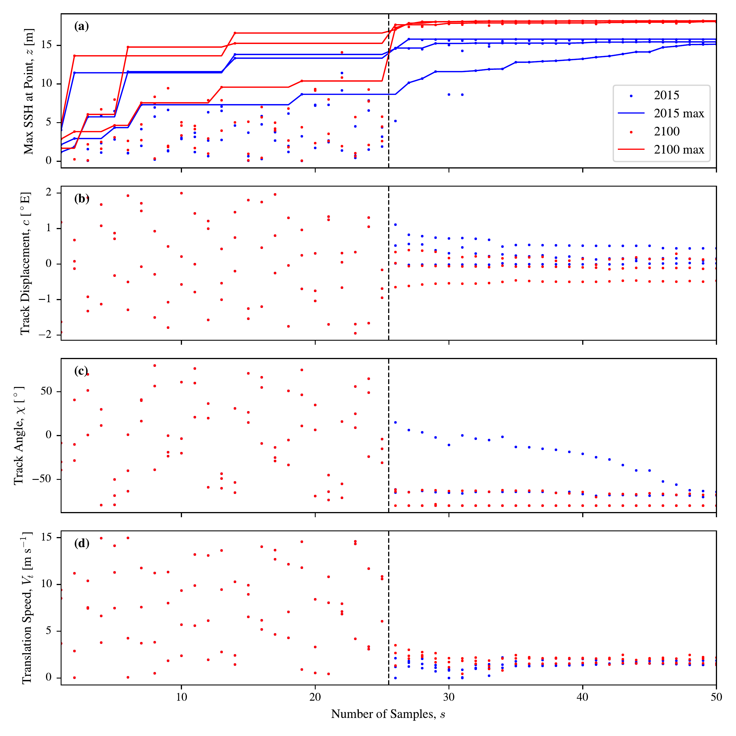
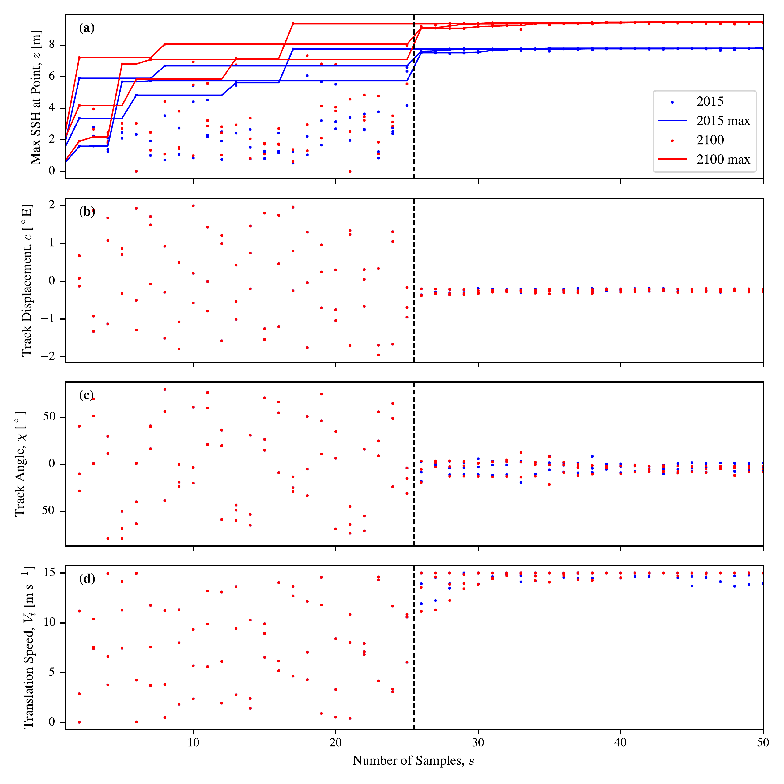
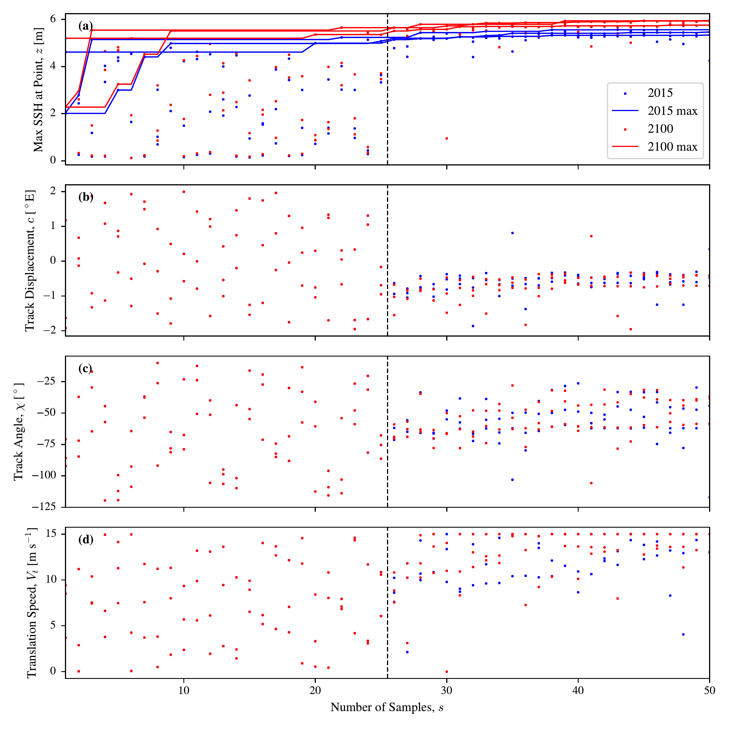
To assess the reliability of finding the potential height and its corresponding optimal trajectory from Figure 4.1, we use the Bayesian optimization framework to find the potential height for different points on the US coastline, repeating each experiment three times with different random seeds, and for both 2015 and 2100 conditions. Using different random seeds results in distinct initial sets of 25 Latin hypercube samples (LHS) and different initial values for the GP’s parameters. The results are shown in Figure 4.5 for New Orleans (and in the Appendix Section Section 4.7, Figures 4.28 and 4.29 for Galveston and Miami respectively). The blue line shows the largest potential height (the highest storm surge height found so far) for 2015 during that Bayesian Optimization experiment, and the red shows the same for 2100 conditions. The potential height found is consistently higher for 2100 than 2015, as would be expected by the increase in both the size and intensity of the imposed idealized cyclone (see Table 4.1). Note that these potential heights do not include mean sea-level rise, which under SSP5-8.5 could add a further 0.5–1 m or more by 2100 (Oppenheimer et al. 2019), so the actual flood heights in a future climate would be higher still. The optimal trajectories do not seem to be significantly different between the two Augusts. Figure 4.5 shows that for one trial the highest value is found after a single additional Bayesian Optimization point has been numerically simulated, whereas for other trials they are still finding higher values for each of the additional 25 Bayesian optimization samples.
Figures 4.6, 4.10, 4.14, and 4.21 show snapshots of ADCIRC simulation from the point at which the maximum storm surge height is reached at the observation point for each of the three trials for 2015 and 2100 conditions for New Orleans, Galveston and Miami respectively. The optimal parameters found for each of these experiments are shown in Table 4.3, with the highest value for each location highlighted in bold (shown previously in Figure 4.1). As can be seen graphically, the snapshots highlight that for some locations the exact angle of approach \(\chi\) does not make a large difference, and we can see a cone of uncertainty for Miami (Figure 4.21) of between \(-33^{\circ}\) and \(-58^{\circ}\), whereas for Galveston (Figure 4.14) this cone is smaller, between \(-8^{\circ}\) and \(1^{\circ}\). New Orleans (Figures 4.6 and 4.10) has a moderate \(\chi\) sensitivity with a range between \(-68.8^{\circ}\) and \(-80^{\circ}\), although this could partly be due to the constraint on \(\chi\) for New Orleans. For these repeats (Figures 4.6 and 4.10), the trajectory travels so that the TC’s RHS roughly pushes water down the channel known as Lake Borgne, which enables the water to be piled up at the observation point (shown as a blue dot).
| Name | Year | Trial | \(i\) | \(c\) [\(^{\circ}\)E] | \(\chi\) [\(^{\circ}\)] | \(V_t\) [m s\(^{-1}\)] | \(z^{*}\) [m] |
|---|---|---|---|---|---|---|---|
| New Orleans | 2015 | 0 | 47 | 0.150664 | -68.583395 | 1.547884 | 15.455311 |
| 2015 | 1 | 26 | -0.024005 | -80.000000 | 1.225401 | 15.810684 | |
| 2015 | 2 | 49 | 0.443851 | -64.282176 | 1.394231 | 15.150438 | |
| New Orleans | 2100 | 0 | 48 | 0.128358 | -67.692634 | 2.230662 | 18.073754 |
| 2100 | 1 | 48 | -0.134150 | -80.000000 | 1.574318 | 18.180207 | |
| 2100 | 2 | 38 | -0.499875 | -80.000000 | 2.076426 | 18.167737 | |
| Galveston | 2015 | 0 | 49 | -0.239934 | -6.546827 | 13.934525 | 7.808678 |
| 2015 | 1 | 46 | -0.202530 | 1.388188 | 14.135774 | 7.784917 | |
| 2015 | 2 | 37 | -0.242096 | -4.413026 | 15.000000 | 7.792348 | |
| Galveston | 2100 | 0 | 41 | -0.260462 | -7.956457 | 15.000000 | 9.456821 |
| 2100 | 1 | 40 | -0.219618 | -1.623654 | 15.000000 | 9.451374 | |
| 2100 | 2 | 38 | -0.228618 | -4.128352 | 15.000000 | 9.449851 | |
| Miami | 2015 | 0 | 49 | -0.474863 | -58.696815 | 15.000000 | 5.337554 |
| 2015 | 1 | 49 | -0.414894 | -44.251724 | 13.009463 | 5.467047 | |
| 2015 | 2 | 42 | -0.339169 | -33.298199 | 13.140890 | 5.561214 | |
| Miami | 2100 | 0 | 46 | -0.645725 | -57.052325 | 15.000000 | 5.756896 |
| 2100 | 1 | 44 | -0.401420 | -37.599006 | 12.778452 | 5.932592 | |
| 2100 | 2 | 49 | -0.403765 | -36.752923 | 13.056293 | 5.952213 |


4.3.3 GP Kernel Sensitivity Analysis
The choice of covariance kernel is a critical design decision in any GP-based model, as it encodes prior assumptions about the function’s smoothness (Rasmussen and Williams 2006). To assess this, we perform a kernel comparison using a dataset of 787 sample locations generated via Latin hypercube sampling, and numerically simulated in high-resolution ADCIRC simulations for the New Orleans location with the 2015 idealized cyclone. Each point in this dataset has the three input parameters (translation speed \(V_t\), track angle \(\chi\), and track displacement, \(c\)), and the resulting maximum storm surge height at the observation point, \(y\).
We repeatedly split the dataset into a small training set of 25 points (mimicking the initial design in a BO run) and a large test set of the remaining 762 points. This should evaluate how well they will model the space at the start of the Bayesian optimization loop. If they are better surrogate models, we expect the Bayesian optimization loop to better estimate potential height. We then train GP models with various kernels and evaluate their predictive performance on the test set using three metrics: the mean predictive log-likelihood (\(\bar{\mathcal{L}}\)) for probabilistic predictions, Root Mean Squared Error (RMSE), a widely used measure of deterministic prediction accuracy, and the coefficient of determination (\(r^2\)) for a scaled score of deterministic accuracy that does not depend on the scale of the predictions. The experiment is repeated over \(N=500\) random train/test splits to ensure statistical robustness. Because the standard error of the mean scales as \(1/\sqrt{N}\), using 500 splits yields standard errors of approximately 0.01 for \(\bar{\mathcal{L}}\) and 0.005 for \(r^2\) (see Table 4.4), which are substantially smaller than the differences between kernel families and therefore sufficient to distinguish their performance.
We summarise the results in Table 4.4. The Matérn family of kernels, which allows for tunable smoothness, consistently outperforms the infinitely smooth squared-exponential (SE) kernel. The Matérn-3/2 kernel achieved the highest mean predictive log-likelihood (\(\bar{\mathcal{L}}=-2.219\pm0.011\)), indicating that it has the best probabilistic fit for the data. The Matérn-5/2 kernel yielded the best deterministic performance, with the lowest RMSE (\(2.281\pm0.015\text{ m}\)) and highest \(r^2\) (\(0.660 \pm 0.005\)). However, the difference between either kernel choice (Matérn-5/2 or Matérn-3/2, both with a zero mean function), is small, indicating that they are both reasonable choices if you are prioritising the mean prediction or the probabilistic prediction. For the Bayesian optimization task, it is probably more important to have accurate probabilistic predictions, so the Matérn-3/2 could be a small improvement. Both kernels significantly outperform the SE and Polynomial kernels, suggesting that the assumption of infinite smoothness is inappropriate for the storm surge response surface, which likely contains sharp gradients as found in other studies such as Gopinathan et al. (2021).
| Kernel | Mean Function | \(\bar{\mathcal{L}}\) | RMSE [m] | \(r^2\) |
|---|---|---|---|---|
| Matérn-\({5}/{2}\) | Constant | -2.254 \(\pm\) 0.015 | 2.294 \(\pm\) 0.016 | 0.656 \(\pm\) 0.005 |
| Matérn-\({5}/{2}\) | Zero | -2.246 \(\pm\) 0.014 | 2.281 \(\pm\) 0.015 | 0.660 \(\pm\) 0.005 |
| Matérn-\({3}/{2}\) | Constant | -2.225 \(\pm\) 0.011 | 2.302 \(\pm\) 0.015 | 0.654 \(\pm\) 0.005 |
| Matérn-\({3}/{2}\) | Zero | -2.219 \(\pm\) 0.011 | 2.292 \(\pm\) 0.015 | 0.657 \(\pm\) 0.005 |
| Matérn-\({1}/{2}\) | Constant | -2.295 \(\pm\) 0.006 | 2.464 \(\pm\) 0.014 | 0.606 \(\pm\) 0.004 |
| Matérn-\({1}/{2}\) | Zero | -2.290 \(\pm\) 0.006 | 2.455 \(\pm\) 0.013 | 0.609 \(\pm\) 0.004 |
| SE | Constant | -2.382 \(\pm\) 0.025 | 2.330 \(\pm\) 0.016 | 0.645 \(\pm\) 0.005 |
| SE | Zero | -2.365 \(\pm\) 0.024 | 2.312 \(\pm\) 0.015 | 0.651 \(\pm\) 0.005 |
| Polynomial | Constant | -2.529 \(\pm\) 0.013 | 2.892 \(\pm\) 0.021 | 0.451 \(\pm\) 0.008 |
| Polynomial | Zero | -2.512 \(\pm\) 0.012 | 2.851 \(\pm\) 0.020 | 0.467 \(\pm\) 0.008 |
4.4 Discussion and Future Work
4.4.1 Findings
The key findings from Section Section 4.3 can be summarized as follows:
The sensitivity of the final potential height to the random seed varies by location. For Galveston, the variation is minimal (c. 0.03 m), while for New Orleans, the spread can be more significant (up to 0.66 m), suggesting the presence of distinct local optima with similar surge magnitudes. This suggests that random error in the solution is low, and so other sources of uncertainty made in the framework in e.g. the low resolution of the ADCIRC model, ignoring wave effects, the idealized CLE15 TC model, and the potential size derivation, are all likely to be more significant. It also suggests that the random error is small enough, so that on its own it would not make potential height less informative for EVT fits (see Chapter 3, Section Section 3.3, Figure 3.11).
However, the random error is more significant for the optimal trajectory found. This difference highlights that there can be local optima that have relatively similar potential heights. It might also imply that the acquisition function we are using (Max-value Entropy Search) may not be the best choice for this problem, as it is designed to find the maximum value rather than its location (Wang and Jegelka 2017). We could instead use the Entropy Search acquisition function (Hennig and Schuler 2012), which is designed to find the location of the maximum with a similar information-theoretic approach. However, this error is not large enough to conflict with our general findings that faster translation speeds are optimal for open coastlines, and slower speeds for enclosed bays, and that the angle of attack can be influenced by the opening of the bay (as for New Orleans Figure 4.2).
There is relatively little difference in the optimal trajectories found between 2015 and 2100 conditions, even though the potential height is consistently higher for 2100, as would be expected by the increase in both the size and intensity of the imposed idealized TCs. This suggests that it may be unnecessary to re-run the Bayesian optimization for different climate conditions, and that a simpler approach of running a single optimization for one climate condition and then re-evaluating the potential height for different climate conditions with a single ADCIRC run may be sufficient. This would be a significant saving in computational cost. In part, this is because we do not include any sea level rise or coastal change within our model, and it is plausible that if both are included the optimal trajectory could change more significantly between the two dates.
The kernel comparison in Section Section 4.3.3, Table 4.4 shows that the choice of kernel has a significant impact on the predictive performance of the GP surrogate model. The Matérn kernels, which allow for tunable smoothness, outperform the standard squared-exponential kernel, suggesting that the storm surge response surface contains sharp gradients that are not well-captured by infinitely smooth assumptions.
4.4.2 Limitations
In Section Section 4.3, we found that the optimal trajectory for New Orleans consistently approached at the angular limit of \(-80^{\circ}\) (travelling roughly westward, deflected 10\(^{\circ}\) northward from due west), while for Galveston and Miami, the optimal translation speed was often at the upper limit of \(15 \text{ m s}^{-1}\). Potential height was also reached near \(V_t\approx 15 \text{ m s}^{-1}\) for Galveston and Miami. This means that the limits that we impose on the BO loop could be important in determining the potential height found, as if a larger range had been allowed, the potential height found could have been even larger.
For New Orleans, the angular limit of \(-80^{\circ}\) to \(80^{\circ}\) is chosen so that the TC approaches from the ocean, with the coastline roughly orientated as a line of constant latitude. TCs can sometimes skim the coastline (e.g. Typhoon Ragasa in 2025), but if the TC spends a significant portion of the approach partially on land, then this should likely reduce the plausible intensity and size of the TC (not modelled here, as we choose a single ocean point at which to calculate potential intensity and size for each location).
However, the choice of TC translation speed is much less certain, as it is chosen to be large compared to the climatology of TC translation speeds in the Atlantic from IBTrACS, and roughly twice the landfall speed of Hurricane Katrina in 2005. However, we have no explicit theory for how translation speed should interact with the potential intensity and potential size, and further work could be done to consider how to integrate the somewhat incompatible assumptions made in Chapter 2 that we are both at a steady equilibrium with the environment (not moving), but that the sea surface temperature and outflow temperature are kept at ambient conditions (which would need the storm to move fast enough to not significantly cool the ocean below it etc.). Considering the TC trade-off between speed, size and intensity could be an important area of future theoretical work.
4.4.3 Future Work
The performance and reliability of the potential height BO framework depend on several key design choices. Our kernel analysis in Section Section 4.3 highlights one such sensitivity, but also confirms that our previous choice was reasonable. Building on this, we identify several critical areas for future research to enhance the methodology.
4.4.3.0.1 Acquisition Functions.
Our current framework uses Max-Value Entropy Search (MES) (Wang and Jegelka 2017), an information-theoretic acquisition function. While powerful, it is important to compare its performance against other established functions. Expected Improvement (EI) (Jones et al. 1998) is a classic choice that focuses on direct improvement, and was used in the TC track optimization study Ide et al. (2024), while Upper Confidence Bound (UCB) (Srinivas et al. 2010) offers theoretical regret guarantees and explicit control over the exploration-exploitation trade-off. Recent work has shown that EI can be viewed as an approximation to MES, suggesting a deeper connection between these philosophies (Cheng et al. 2025). A systematic comparison of these functions, particularly in a batch setting (e.g., q-UCB), is needed to determine the most efficient strategy for the storm surge problem. We conduct some preparatory experiments with EI in Section Section 4.6, Table 4.5, Table 4.6, but a more thorough comparison is needed.
4.4.3.0.2 Noise Modeling.
We currently assume a small, fixed noise term to account for numerical artifacts in the ADCIRC simulation. However, the simulation is largely deterministic. Comparing this noisy assumption against a noise-free GP model is an important step. A noise-free model could fit the observed data more closely but risks overfitting, while a small “nugget” term can improve numerical stability and robustness (Rasmussen and Williams 2006). Investigating the impact of this choice on convergence speed and final optima is a key research question.
4.4.3.0.3 Informative Priors.
The standard GP assumes a zero-mean prior, learning the function’s behavior entirely from the data. This can be inefficient if prior physical knowledge is available. An alternative is to use an informative prior mean function (as shown for particle physics in Boltz et al. 2025), for example, derived from a faster, lower-fidelity surge model or an empirical formula (Mori et al. 2022, used a simple empirical formula (response function) and \(V_p\) to calculate their “maximum potential surge”). Such a “gray-box” approach could significantly accelerate convergence by guiding the initial search towards physically plausible high-surge regions, while retaining the ability to numerically simulate the full complexity of the coast.
4.4.3.0.4 Advanced Geometries and Physics.
The current work is limited to straight-line TC tracks. Extending the optimization space to include track curvature, as explored by Ide et al. (2024), would allow for the discovery of more complex and potentially more hazardous scenarios. Furthermore, our analysis only considers the peak surge at a single point. Expanding the framework to a multi-objective problem (Kandasamy et al. 2017), optimizing for maximum surge across a stretch of coastline or considering other impacts like wave height, would provide a more comprehensive hazard assessment. We might be able to leverage observational data (e.g. IBTrACS), but historical tracks do not directly define a continuous parameter space from which the BO loop can sample. Two avenues could bridge this gap: training a generative model on IBTrACS to produce realistic tracks from a small number of latent inputs, or extending the parameterisation to include additional degrees of freedom (e.g. track curvature, time-varying intensity) so that observed track variability is better represented in the search space.
4.5 Conclusion
This work demonstrates that Bayesian optimization is a powerful and efficient tool for identifying the potential height of tropical cyclone storm surges, a critical task for coastal risk assessment in a changing climate. Our application of the framework to diverse US coastal locations successfully identified physically plausible high-impact scenarios that are sensitive to both local geography and future climate conditions.
A key contribution of this work is the systematic evaluation of Gaussian Process kernels, which showed that the smoothness assumptions encoded in the kernel have a significant impact on predictive accuracy. The superior performance of Matérn kernels over the standard squared-exponential kernel provides valuable guidance for practitioners modeling similar complex physical systems. The outlined directions for future work, particularly concerning the choice of acquisition function and the incorporation of prior physical knowledge, promise to further enhance the power and reliability of this data-centric approach to understanding extreme environmental events.
Open source code
The code for this work is available at https://github.com/sdat2/PotentialHeight (Thomas 2025), and
builds upon the trieste library (Picheny et
al. 2023) and the sithom utility library
(Thomas
2024).
4.6 Appendix: Additional Bayesian Optimization Results
In Table 4.5 we show the optimal TC parameters found for the potential height for New Orleans, Galveston and Miami, for 2015 and 2100 conditions with multiple repeats with the EI DAF. This can be compared to Table 4.6 which shows the same results for the MES DAF, for a greater number of repeats. If we plot the full experiments we should be able to better estimate the ability of each DAF to find the potential height quickly and reliably (i.e. minimize simple regret).
| Name | Year | Trial | \(i\) | \(c\) [\(^{\circ}\)] | \(\chi\) [\(^{\circ}\)] | \(V_t\) [m s\(^{-1}\)] | \(z^{*}\) [m] |
|---|---|---|---|---|---|---|---|
| New Orleans | 2015 | 0 | 35 | 0.106144 | -65.765142 | 2.645223 | 16.623703 |
| 2015 | 1 | 27 | -0.037976 | -72.105791 | 2.610292 | 16.646118 | |
| 2015 | 2 | 34 | 0.080311 | -73.216037 | 2.137189 | 16.568913 | |
| 2015 | 3 | 48 | 0.178416 | -50.576019 | 3.424609 | 16.197922 | |
| New Orleans | 2100 | 0 | 34 | 0.116110 | -64.564155 | 2.502893 | 19.005556 |
| 2100 | 1 | 9 | 0.188782 | -74.528809 | 3.266373 | 17.358231 | |
| 2100 | 2 | 50 | 0.081534 | -72.808089 | 1.050691 | 18.617483 | |
| 2100 | 3 | 11 | 0.532410 | -38.566895 | 6.979294 | 12.756316 | |
| Miami | 2015 | 0 | 50 | -0.907845 | -65.559199 | 14.199726 | 5.808904 |
| 2015 | 1 | 45 | -0.755691 | -58.689019 | 12.467778 | 5.855880 | |
| 2015 | 2 | 42 | -0.317724 | -14.295937 | 15.000000 | 5.878907 | |
| 2015 | 3 | 44 | -0.493195 | -42.803518 | 9.394865 | 5.804811 | |
| 2015 | 4 | 47 | -0.436209 | -42.899324 | 14.359218 | 6.025050 | |
| Miami | 2100 | 0 | 50 | -1.089736 | -64.441735 | 14.217393 | 6.275769 |
| 2100 | 1 | 46 | -0.812193 | -59.644524 | 13.642048 | 6.352571 | |
| 2100 | 2 | 48 | -0.516151 | -41.709921 | 15.000000 | 6.469617 | |
| 2100 | 3 | 48 | -0.505128 | -41.683116 | 9.644382 | 6.181484 | |
| 2100 | 4 | 45 | -0.581573 | -44.306367 | 14.214715 | 6.439702 | |
| Galveston | 2015 | 0 | 49 | -0.403830 | -21.338870 | 8.279774 | 8.286314 |
| 2015 | 1 | 45 | -0.350905 | -12.918042 | 14.575252 | 9.227775 | |
| 2015 | 2 | 47 | -0.356173 | -17.930728 | 14.526479 | 9.264994 | |
| 2015 | 3 | 50 | -0.302235 | -16.091937 | 10.399270 | 8.754756 | |
| 2015 | 4 | 50 | -0.535234 | -38.618675 | 8.980126 | 8.285849 | |
| Galveston | 2100 | 0 | 50 | -0.414398 | -24.336226 | 8.494458 | 10.055245 |
| 2100 | 1 | 41 | -0.374471 | -16.827473 | 14.330211 | 11.007732 | |
| 2100 | 2 | 42 | -0.391046 | -20.149699 | 14.586575 | 11.015003 | |
| 2100 | 3 | 48 | -0.355822 | -15.085349 | 10.537436 | 10.511299 | |
| 2100 | 4 | 45 | -0.620599 | -36.978461 | 9.332306 | 10.008612 |
| Name | Year | Trial | \(i\) | \(c\) [\(^{\circ}\)] | \(\chi\) [\(^{\circ}\)] | \(V_t\) [m s\(^{-1}\)] | \(z^{*}\) [m] |
|---|---|---|---|---|---|---|---|
| New Orleans | 2015 | 0 | 48 | 0.150664 | -68.583395 | 1.547884 | 15.455311 |
| 2015 | 1 | 27 | -0.024005 | -80.000000 | 1.225401 | 15.810684 | |
| 2015 | 2 | 50 | 0.443851 | -64.282176 | 1.394231 | 15.150438 | |
| 2015 | 3 | 49 | 0.435980 | -79.011548 | 0.814035 | 15.760807 | |
| 2015 | 4 | 48 | 0.061778 | -69.469572 | 2.117449 | 16.331021 | |
| 2015 | 5 | 50 | 0.032803 | -80.000000 | 1.274389 | 16.346804 | |
| 2015 | 6 | 42 | -0.296418 | -80.000000 | 1.688346 | 16.401895 | |
| 2015 | 7 | 27 | 0.190199 | -65.280805 | 2.360441 | 16.256331 | |
| 2015 | 8 | 45 | -0.292706 | -80.000000 | 1.560420 | 16.415911 | |
| 2015 | 9 | 50 | 0.500926 | -9.271796 | 2.309178 | 13.210543 | |
| 2015 | 10 | 50 | 0.192714 | -60.737065 | 2.891723 | 16.203676 | |
| 2015 | 11 | 48 | 0.277146 | -75.769189 | 1.365527 | 16.150175 | |
| New Orleans | 2100 | 0 | 49 | 0.128358 | -67.692634 | 2.230662 | 18.073754 |
| 2100 | 1 | 49 | -0.134150 | -80.000000 | 1.574318 | 18.180207 | |
| 2100 | 2 | 39 | -0.499875 | -80.000000 | 2.076426 | 18.167737 | |
| 2100 | 3 | 50 | 0.184383 | -61.389076 | 1.685182 | 18.433191 | |
| 2100 | 4 | 50 | 0.113350 | -67.124205 | 2.231882 | 18.678784 | |
| 2100 | 5 | 14 | 0.313660 | -64.816895 | 5.924606 | 12.823672 | |
| 2100 | 6 | 39 | 0.165419 | -59.671687 | 3.118457 | 18.771043 | |
| 2100 | 7 | 1 | -0.073730 | -61.308594 | 2.074585 | 17.684511 | |
| 2100 | 8 | 38 | -0.333299 | -80.000000 | 1.514461 | 18.738474 | |
| 2100 | 9 | 3 | 1.586426 | 47.285156 | 3.143921 | 7.072265 | |
| 2100 | 10 | 45 | 0.158070 | -60.216438 | 3.126566 | 18.787441 | |
| 2100 | 11 | 3 | 0.591370 | 65.363770 | 2.534866 | 9.210907 | |
| Miami | 2015 | 0 | 50 | -0.474863 | -58.696815 | 15.000000 | 5.337554 |
| 2015 | 1 | 50 | -0.414894 | -44.251724 | 13.009463 | 5.467047 | |
| 2015 | 2 | 43 | -0.339169 | -33.298199 | 13.140890 | 5.561214 | |
| 2015 | 3 | 35 | -0.384161 | -29.815032 | 14.667681 | 5.629461 | |
| 2015 | 4 | 46 | -0.744002 | -59.949934 | 9.760519 | 5.339923 | |
| 2015 | 5 | 39 | -0.873098 | -60.735722 | 8.801652 | 5.295642 | |
| 2015 | 6 | 46 | -0.627557 | -54.849255 | 12.125315 | 5.411477 | |
| 2015 | 7 | 36 | -0.463462 | -38.612121 | 13.576390 | 5.620397 | |
| 2015 | 8 | 44 | -0.509733 | -51.497712 | 8.433675 | 5.369272 | |
| 2015 | 9 | 4 | -0.413574 | -32.714844 | 10.643921 | 5.571131 | |
| 2015 | 10 | 10 | -0.299561 | -23.173828 | 10.701599 | 5.680423 | |
| 2015 | 11 | 46 | -0.318434 | -28.584325 | 13.558010 | 5.647601 | |
| Miami | 2100 | 0 | 47 | -0.645725 | -57.052325 | 15.000000 | 5.756896 |
| 2100 | 1 | 45 | -0.401420 | -37.599006 | 12.778452 | 5.932592 | |
| 2100 | 2 | 50 | -0.403765 | -36.752923 | 13.056293 | 5.952213 | |
| 2100 | 3 | 37 | -0.404466 | -33.068057 | 14.413090 | 6.051083 | |
| 2100 | 4 | 50 | -0.759946 | -57.534220 | 14.095991 | 5.826954 | |
| 2100 | 5 | 43 | -0.922258 | -58.354497 | 9.329459 | 5.666612 | |
| 2100 | 6 | 46 | -0.732460 | -53.882079 | 9.551218 | 5.809021 | |
| 2100 | 7 | 44 | -0.501872 | -38.525615 | 14.078191 | 6.022338 | |
| 2100 | 8 | 24 | -1.145447 | -67.741699 | 6.491776 | 5.557811 | |
| 2100 | 9 | 4 | -0.413574 | -32.714844 | 10.643921 | 5.946936 | |
| 2100 | 10 | 50 | -0.385609 | -29.661194 | 11.205281 | 6.023767 | |
| 2100 | 11 | 48 | -0.357789 | -22.981955 | 13.741247 | 6.076998 | |
| Galveston | 2015 | 0 | 50 | -0.239934 | -6.546827 | 13.934525 | 7.808678 |
| 2015 | 1 | 47 | -0.202530 | 1.388188 | 14.135774 | 7.784917 | |
| 2015 | 2 | 38 | -0.242096 | -4.413026 | 15.000000 | 7.792348 | |
| 2015 | 3 | 46 | -0.295615 | -8.472373 | 10.243142 | 7.897922 | |
| 2015 | 4 | 46 | -0.274242 | -9.557076 | 12.083916 | 8.117956 | |
| 2015 | 5 | 43 | -0.315450 | -21.033440 | 9.173075 | 7.755775 | |
| 2015 | 6 | 50 | -0.338784 | -19.658241 | 9.593588 | 7.830658 | |
| 2015 | 7 | 49 | -0.341349 | -15.711692 | 11.881489 | 8.107960 | |
| 2015 | 8 | 42 | -0.343098 | -24.416809 | 7.671206 | 7.521423 | |
| 2015 | 9 | 49 | -0.337953 | -22.515926 | 9.835710 | 7.837834 | |
| 2015 | 10 | 50 | -0.356872 | -20.149886 | 10.369618 | 7.930439 | |
| 2015 | 11 | 28 | -0.227945 | -1.538035 | 13.293142 | 8.148791 | |
| Galveston | 2100 | 0 | 42 | -0.260462 | -7.956457 | 15.000000 | 9.456821 |
| 2100 | 1 | 41 | -0.219618 | -1.623654 | 15.000000 | 9.451374 | |
| 2100 | 2 | 39 | -0.228618 | -4.128352 | 15.000000 | 9.449851 | |
| 2100 | 3 | 50 | -0.304825 | -4.035788 | 11.587170 | 9.636491 | |
| 2100 | 4 | 44 | -0.293576 | -6.798316 | 12.710099 | 9.812594 | |
| 2100 | 5 | 46 | -0.337807 | -22.121024 | 8.961768 | 9.351685 | |
| 2100 | 6 | 50 | -0.488446 | -24.842308 | 9.343398 | 9.301671 | |
| 2100 | 7 | 47 | -0.366055 | -23.211359 | 9.987884 | 9.516553 | |
| 2100 | 8 | 48 | -0.368090 | -26.706469 | 8.476046 | 9.216771 | |
| 2100 | 9 | 49 | -0.394500 | -21.304301 | 9.912835 | 9.523946 | |
| 2100 | 10 | 50 | -0.384730 | -20.524362 | 10.385365 | 9.584086 | |
| 2100 | 11 | 28 | -0.234762 | -2.492068 | 13.252825 | 9.804772 |
4.7 Additional Bayesian Optimization Process Figures
Figures 4.28 and 4.29 are additional figures that show the same Bayesian optimization process as Figure 4.5, but for Galveston and Miami respectively. As before, the first 25 points before the dashed black line are for the Latin hypercube search sampling strategy, and the remaining 25 points are selected with the MES acquisition function. The blue points are for 2015 conditions, and the red points for 2100 conditions. Each experiment is repeated three times with different random seeds. The final potential height found is indicated by the dashed horizontal line of the same color.
References
\(\chi \in \left(-80, 80\right)\) for New Orleans, \(\chi \in \left(-80, 80\right)\) for Galveston, \(\chi \in \left(-120, 10\right)\) for Miami↩︎
Both the PI potential outer size \(r_{a3}\) for the radius of vanishing wind, and the PI potential inner size \(r_3\) for the radius of maximum wind, both calculated for the intensity equal to the potential intensity.↩︎