Chapter 3
Finding the potential height of tropical storm surges in a changing climate using Bayesian optimization
Note: This Chapter is under review with Environmental Data Science (EDS) since March 2025. A preprint is available at: https://doi.org/10.31223/X57T5R. The work is presented here with slight modifications to fit the thesis format. This was conducted before Chapter 2, and so uses a less efficient method of calculating the potential size than that presented in Chapter 2. It also uses slightly different terminology (‘Carnot engine’ for the W22 cycle rather than the more accurate ‘sub-Carnot’ description). The author list is Simon D.A. Thomas, Dani C. Jones, Talea Mayo, John R. Taylor, Henry B. Moss, David R. Munday, Ivan D. Haigh, Devaraj Gopinathan. All the work was primarily done by Simon D.A. Thomas as part of this PhD thesis, and all other authors were supervisors or collaborators, providing advice and/or editing.
Abstract. We introduce a new framework for systematically exploring the largest storm surge heights that a tropical cyclone (TC) in a given climate can create. We calculate the TC potential intensity and the potential size from climate model projections and find that both these limits increase in response to climate change. We then use Bayesian optimization with a barotropic ocean circulation model to find the maximum height that the surge can reach given these limits. The key methodological advances of this paper are (i) calculation of the recently proposed potential size of a TC, now and under climate change (ii) using Bayesian optimization to find the largest storm surge given those constraints, (iii) using this information to constrain the return level curve. This paper uses key theoretical improvements in our understanding of TCs to understand implications for changing storm surge risk. We have chosen the US coastline and the area around New Orleans as our case study area, but this method is generalizable and could in principle be applied to any coastline.
Impact Statement. Our methodology provides a way of assessing the impact of climate change on storm surges. We calculate previously proposed upper bounds on the intensity and size of a tropical cyclone given the climate, and then use machine learning to provide an efficient method of calculating the storm surge. By focusing on the worst case storm surge and its relation to the climatic conditions, we can improve predictions of damaging long return period storm surges. Our novel approach can easily be transferred to other coastlines around the world that are influenced by tropical cyclones.
3.1 Introduction
Whilst state-of-the-art climate models are invaluable research tools for many questions, they struggle to explicitly resolve TCs. As climate models must parameterize processes that require spatial scales smaller than the lateral grid box spacing (typically 1\(^{\circ}\) in CMIP6 as in CESM2, Danabasoglu et al. (2020)), these small-scale processes (e.g. the eye-wall, rainbands and warm ocean currents) risk being misrepresented (Camargo and Wing 2016). Furthermore, the creation of TCs (cyclogenesis) relies on seeding events such as African easterly waves (AEWs), and a bias in the simulation of these leads to a bias in cyclogenesis (Camargo and Wing 2016). Similarly, there are well-known biases in TC seasonality (Sainsbury et al. 2022; Peng and Guo 2024; Shan et al. 2023), frequency (Sainsbury et al. 2022), intensification (Roberts et al. 2020), and intensity (Roberts et al. 2020) within modern climate models. When storm surge models are then forced with TCs from these models, even with attempts to bias correct them, these biases can be propagated into estimates of the storm surge hazard and resultant risk (e.g. Sobel et al. (2023)).
TCs are also dependent on broad-scale fields such as surface temperature. Along with a finite amplitude genesis event (such as an AEW) (Emanuel 1991), TCs are generated due to a thermodynamic disequilibrium between the sea surface and the tropopause (Emanuel 1986, 2003, 2006). The potential intensity (PI) was introduced by Emanuel (1986), by imagining a Carnot cycle running between these reservoirs, and has been long-accepted as a reasonable measure for the upper bound in TC azimuthal speeds (Rousseau-Rizzi et al. 2021). The potential intensity is expected to increase with climate change as the disequilibrium between reservoirs is increased by the enhanced greenhouse effect, and there is observational evidence that the upper bound of TC intensity has increased over recent years (Wehner and Kossin 2024). Studies have previously used the potential intensity to investigate subsequent limits of resulting storm surge heights (e.g. Mori et al. (2022)). The size of the TC also significantly affects the size of a storm surge, and D. Wang et al. (2022) proposed a new measure of potential size (PS), though it has not yet been used with climate model output or to constrain downstream consequences. Given these two limits (i.e. of potential intensity and potential size), the height of storm surges generated by TCs should be limited, too.
In order to relate these limits of potential size and intensity to a corresponding limit on storm surge height, we can use a storm surge model ADCIRC (Luettich Jr and Westerink 1991) running in a Bayesian Optimization loop. We assume that both PI and PS are achieved at the same time, taking a value from the grid-point nearest that point along the coast at that time, and then as in Jia and Taflanidis (2013) we vary the TC trajectory and speed to find the highest storm surge height that can be created at that point. This helps to incorporate the complex interplay between the bathymetry and storm surge trajectory in a flexible and efficient way, and Ide et al. (2024) showed that Bayesian optimization can effectively find the most impactful TC trajectory for a storm surge. Mori et al. (2022) used the calculated potential intensity together with coastal response functions (Irish et al. 2009) instead of a full storm surge model to show that the potential storm surge height increased, with a study area of bays in East Asia, but although using response functions is likely more efficient, this may not fully account for the effects of complex coastal geometry, and they were not able to include the potential size change in TCs from D. Wang et al. (2022). On the other hand, Lin and Emanuel (2016) ran the ADCIRC model with very large catalogues of realistic TCs to estimate the long return period “Grey Swan” TC storm surges for numerous points around the world. This is likely much more computationally intensive, but allows for more complex TC trajectories.
Understanding the worst-case storm surge, which we choose to call the potential height, is useful for several reasons. The design requirements for critical infrastructure and emergency response and planning efforts rely on estimates of low probability and worst-case scenarios. Some structures are designed to withstand very high return period events (e.g. coastal nuclear power plants Schwerdt et al. (1979; ONR 2014), which are designed to withstand a one in a 10,000 year storm surge), and having an estimate of the potential height may be an efficient way of informing the design requirements. Beyond the worst case itself, knowledge of the potential height provides a physically grounded upper bound that can constrain extreme value distributions, thereby improving the estimation of high-return-period events (e.g. 1-in-100 or 1-in-500 year storm surges) even when observational records are short.
The framework we introduce here can be extended to other coastlines around the world that are influenced by TCs. Our work is novel in three ways:
Calculating TC potential size using climate data, both in the present and future (which builds upon D. Wang et al. (2022, 2023)).
Using Bayesian optimization to find the worst possible storm surge from the potential intensity and potential size limits.
Using this worst-case estimate and extreme value theory to demonstrate how they can reduce uncertainties in the return period curve.
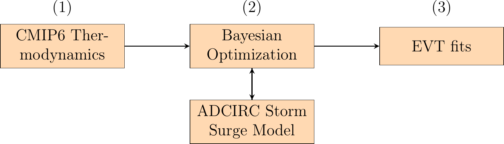
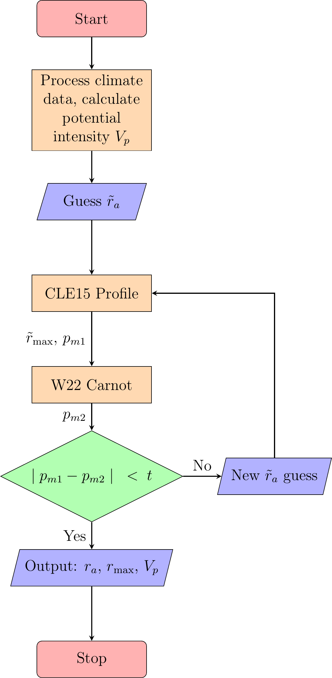
We first discuss our proposed framework (Section Section 3.2) and explain how the potential intensity (PI) and potential size (PS) thermodynamic limits are calculated (Section Section 3.2.2). We then describe the climate data used to calculate these limits, and the methods used to process them (Section Section 3.2.1). We explain how the ADCIRC model is used to calculate the storm surge (Section Section 3.2.3). In Section Section 3.2.4 we describe how Bayesian optimization is used to find the worst-case storm surge. Finally, we explain how extreme value theory is used to find the return period curve (Section Section 3.2.5). This method is shown as a flowchart in Figure 3.1. We present our results in Section Section 3.3. We first show how we can optimize for one point along the coast, and then demonstrate how we can extend our finding to many points along the coast to understand how the maxima and the characteristics of the maxima vary spatially and over time. We then discuss the utility and limitations of this approach (Section Section 3.4). We conclude our study and summarise our key results in Section Section 3.5. To aid readability, abbreviations have been listed in Table 3.1.
| Abbreviation | Expansion |
|---|---|
| TC | Tropical cyclone |
| PI | TC potential intensity (Emanuel 1986) |
| PS | TC potential size (D. Wang et al. 2022) |
| CLE15 | Chavas et al. (2015)’s TC wind profile |
| W22 | D. Wang et al. (2022) Carnot engine |
| GP | Gaussian process |
| DAF | Data acquisition function |
| MES | Max-value entropy search (Wang and Jegelka 2017) |
| EVT | Extreme value theory |
| GEV | Generalized extreme value distribution |
| CMIP6 | Coupled Model Intercomparison Project Phase 6 |
| ADCIRC | ADvanced CIRCulation model |
3.2 Methodology
3.2.1 Climate data
The potential intensity and potential size limits can be calculated based on the output of climate models, which will allow us to explore how these limits might evolve in the future. From the current state-of-the-art collection of climate models, CMIP6, we can use the historical experiments for plausible realisations of the past climate from 1850-2014, and the SSP-585 scenario, the most pessimistic scenario of those developed for 2015-2100. While SSP-585 may not be the most likely outcome given recent progress in renewable energy (Huard et al. 2022), it provides a large warming signal difference that should make it easier as a first test of our techniques. We have chosen to use the CMIP6 models included in the Pangeo data catalogue’s Google Cloud Store (Pangeo 2022) because this data is easily available. We have initially chosen to focus on an ensemble member of the CESM2 climate model (Danabasoglu et al. 2020) but the analysis could be simply extended to any of the other models in the catalogue. The data from the Pangeo catalogue is preprocessed using the xMIP preprocessing package (Busecke et al. 2023), which ensures the ensemble members are all converted to SI units and compatible label names. The data is then regridded to \(\frac{1}{2}^{\circ}\) using CDO (Schulzweida 2023). Initially we have not implemented a method of bias correction either for the mean state or trend (as in Mori et al. (2022)), but we would like to explore the effects of bias correction in the future on both measures.
3.2.2 Potential intensity and potential size
We use the TC potential intensity first proposed in Emanuel (1986), in its most common formulation as a measure of the maximum azimuthal windspeed attainable (as reviewed in Rousseau-Rizzi et al. (2021)).
This is calculated following Bister and Emanuel (2002) as \[\begin{equation} \left(V_{p}\right)^2 = \frac{T_s}{T_0}\frac{C_k}{C_D} \left(\text{CAPE}^{*} - \text{CAPE}_{\mathrm{env}}\right)\mid_{RMW}, \end{equation}\](3.1) where \(V_{p}\) is the potential intensity at the gradient wind level (\(V_{\mathrm{reduc}}=1\) in Gilford (2021)), \(\text{CAPE}^{*}\) is the convective available potential energy of saturated air lifted from the sea surface to the outflow level, \(\text{CAPE}_{\mathrm{env}}\) is the convective available potential energy of the environment, \(C_K\) is the enthalpy exchange parameter, \(C_D\) is the momentum exchange parameter, \(T_s\) is the surface temperature, and \(T_o\) is the outflow temperature, and it is evaluated at the radius of maximum winds, \(\mathrm{RMW}\). The tcPyPI provides a user-friendly package for calculating the potential intensity (Gilford 2021), and we assume \(\frac{C_K}{C_D} = 0.9\) which is standard.
Despite the acceptance of the potential intensity of a TC, there has been less success in determining how large a TC can grow. The potential size metric was suggested by D. Wang et al. (2022) based on assuming both an improved Carnot cycle running between the sea surface and the tropopause and the azimuthally symmetric wind and pressure dynamical profile of Chavas et al. (2015). This is reasonable because as the storm becomes larger, the pressure drop modeled by the Carnot cycle is reduced, and the pressure drop assumed by the dynamical profile with cyclogeostrophic balance increases (following Chavas et al. (2017)). There will be one radius of outer winds where both models predict the same pressure drop at a particular storm outer radius (D. Wang et al. 2022). This solution can be found using a method such as the bisection method, finding the point at which the two modeled radii intersect. We assume that the maximum windspeed from the Chavas et al. (2015) profile is the potential intensity \(V_{p}\). We then assume that the maximum windspeed for the D. Wang et al. (2022) W22 Carnot engine, \(V_{\mathrm{max\; W22}}\), is given by the potential intensity multiplied by the supergradient factor \(\gamma_{\mathrm{sg}}=1.2\) of D. Wang et al. (2022). We are therefore assuming that the cyclone is both at its maximum potential intensity \(V_{p}\) and maximum potential size \(r_a\) at the same time.
This potential size \(r_a\) is justified by assuming that if a TC has reached the maximum windspeed under the potential intensity limit, there might still be additional energy (work) that could be extracted by expanding the size of the TC. The point at which the maximum windspeed of the TC can be maximally expanded, whilst satisfying both the dynamical limits from assuming the Chavas et al. (2015) radial profile and assuming the D. Wang et al. (2022)’s updated TC Carnot engine is called the potential size \(r_a\). In their paper this is calculated as the outer radius of vanishing winds (\(r_a\)), but the Chavas et al. (2015) profile with a given velocity of maximum winds \(V_{p}\) has a single radius of maximum winds, \(r_{\mathrm{max}}\), that this would correspond to assuming that the other environmental conditions are held constant. Further details of the potential intensity and size calculation procedure are discussed in Section Section 3.6.
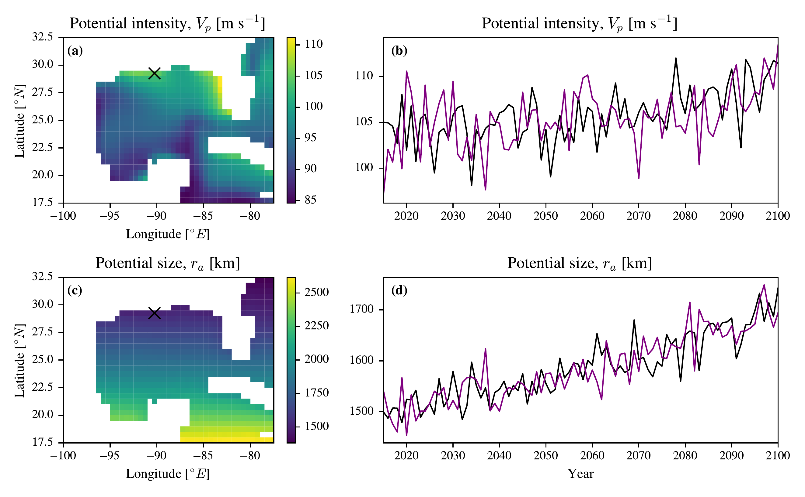
Potential size depends on potential intensity, and both of these quantities depend on the broad-scale climate variables of the atmospheric profile and surface variables at a point. Figures Figure 3.2(a) & (c) show the potential intensity and size calculated on a processed monthly average from a single CMIP6 ensemble member (CESM2-r4i1p1f1) for August 2015. As shown in Figure 3.2(a), potential intensity is higher in areas with higher sea surface temperature (a spatial correlation coefficient of \(\rho=0.97\) between SST and potential intensity, and a linear gradient fit of \(m=11\pm1\) m s\(^{-1}\) \(^{\circ}\)C\(^{-1}\)). Whereas, Figure 3.2(c) shows that geographically potential size is dominated by the north-south contrast (a spatial correlation coefficient of \(\rho=-0.99\) between latitude and potential size (\(m=-88\pm1\) km \(^{\circ}\)N\(^{-1}\))), consistent with the \(\frac{V_{p}}{f}\) scaling in D. Wang et al. (2022) where \(f\) is the Coriolis parameter and \(V_{p}\) is the potential intensity (\(\rho=0.92, m=\left(1.48\pm0.03\right)\times10^{3}\) m rad\(^{-1}\)). Therefore, as might be expected, much larger and more intense TCs are possible in the warmer waters further south.
When we look at a point near New Orleans (29.25\(^{\circ}\)N, -90.25\(^{\circ}\)E) where we have plotted the metrics calculated from monthly average data from CESM2-r4i1p1f1 (black) and CESM2-r10i1p1f1 (purple) for August the SSP-585 (2015-2100) scenarios, the two metrics vary over time in quite different ways (Figure 3.2b&d). Potential intensity (Figure 3.2(b)) shows much higher variability relative to its magnitude than potential size (Figure 3.2d). For r4i1p1f1, over the SSP-585 scenario from 2015-2100 the increase of potential size (\(\rho=0.89\), \(m= 2.3\pm0.1\) km yr\(^{-1}\)) is more visible and significant than potential intensity (\(\rho=0.57\), \(m=\left(6.6\pm1.0\right)\times10^{-2}\) m s\(^{-1}\) yr\(^{-1}\)), where \(\rho\) is the correlation coefficient against time, and \(m\) is the gradient of a linear fit over the period, and we calculate the standard deviation of this parameter based on the fit. Therefore, both of these metrics appear to increase as a response to climate change, but potential size seems to show a more significant effect, which is an interesting property not highlighted in D. Wang et al. (2022). There is a much stronger correlation between the timeseries during SSP-585 at this point for SST and potential size (\(\rho=0.93\), \(m=57\pm3\) km \(^{\circ}\)C\(^{-1}\)) compared to SST and potential intensity (\(\rho=0.70\), \(m=1.9\pm0.2\) m s\(^{-1}\) \(^{\circ}\)C\(^{-1}\)).
3.2.3 ADCIRC model driven by idealized TC
We use the ADCIRC model in the barotropic two-dimensional depth-integrated mode (Luettich et al. 1992; Westerink et al. 1994), which is a state-of-the-art storm surge model solved on an unstructured mesh with triangular elements. ADCIRC solves the generalized wave continuity equation using a Jacobi preconditioned iterative solver (Westerink et al. 1994). Many different meshes are available online to resolve the coastline in a variety of different levels of detail.
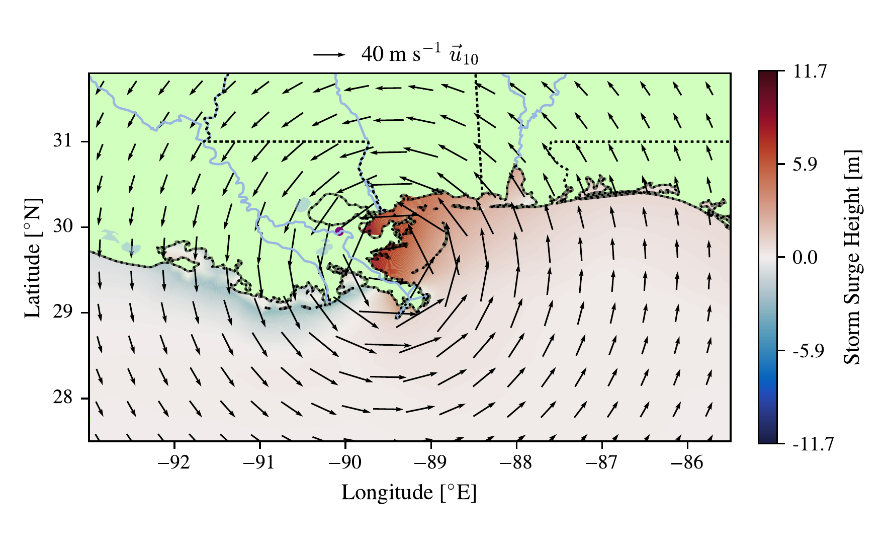
We used the EC95c mesh (Mukai et al. 2002; Blain et al. 1994, 1998), which belongs to the “Eastcoast” family of Western North Atlantic ADCIRC domains (see Szpilka et al. 2016, for a history of the series). The mesh resolves the East and Gulf of Mexico US coastlines using 58,369 triangular elements with 31,435 nodes; element sizes range from roughly 1 km along the coast to approximately 100 km in the deep ocean (see also Dietrich et al. 2013). This resolution captures some small-scale structures of the US such as the barrier islands on the coast. The model lacks some geographic features such as Lake Pontchartrain to the north of New Orleans, and does not allow the water to flow onto the land. We input the atmospheric forcing fields using the netCDF format, with a large stationary grid over the whole domain at a resolution of \(\frac{1}{8}^{\circ}\), and a moving grid centered on the TC center at a resolution of \(\frac{1}{80}^{\circ}\). Both grids are regular, orientated to be parallel to lines of constant latitude and longitude. The ADCIRC setup does not include tides, and has a timestep of five seconds. Further details of the storm surge model mesh and its settings are described in Section Section 3.7. An example snapshot of the model being forced by the CLE15 wind profile for August 2015 is shown in Figure 3.3.
3.2.4 Bayesian Optimization and Surrogate Modelling
In this study, the objective function \(f(\vec{x})\) being maximised is the maximum storm surge height \(z\) (in metres) at a chosen coastal point, as a function of the TC track parameters \(\vec{x} = (\chi, c, V_t)\): the track bearing \(\chi\), the east–west displacement \(c\), and the translation speed \(V_t\).
In Bayesian optimization (Garnett 2023), we seek to find the global optimum of a function \(f\left(\vec{x}^{*}\right)\), where \(f:\;\vec{x} \in \mathbb{R}^N \to z \in \mathbb{R}\). We seek to do this with a minimum number of samples of \(\vec{x}\), \(N_s\), so as to reduce the computational cost of finding \(f\left(\vec{x}^{*}\right)\), especially when \(f\) is computationally expensive. To make repeated evaluations of \(f\) amenable, we replace \(f\) with its inexpensive statistical surrogate \(\hat{f}\) (also known as a meta-model, or emulator). To reduce the total number of samples, as well as to find samples that are most informative of \(f\), we define a data acquisition function (DAF), \(\alpha_t\left(\vec{x}\right)\). The DAF maximises mutual information to find the most informative next sample or samples for \(f\) (or \(\hat{f}\)) after it has been fitted on all of the previous samples.
Bayesian optimization has been widely used in applications where each additional sample is computationally expensive to utilize, e.g. in changing the hyper– and meta– parameters of a deep learning model (Garnett 2023), where retraining a model may take days of computational time. It is also a good approach to replicate simulations from numerical models of physical systems, which can be very expensive and often depend on many parameters that are hard to tune (see e.g. Khatamsaz et al. (2023)).
In our case, \(f(\vec{x})\) is the ADCIRC storm surge model, and the optimisation points \(\vec{x}_s = (\chi, c, V_t)\) are TC track parameters (the inputs to ADCIRC), not hyper-parameters of the GP or the storm-surge model itself. Rather than tuning the parameters of the numerical storm-surge model, we aim to change the characteristics of the idealized TC used to force it. Defining the limits of the TC characteristics \(\vec{x}\), we can sequentially run ADCIRC with different sets of TC characteristics and produce values of the resulting maximum storm surge heights at a point \(z\); to be consistent with the derivation of the potential size, we use the azimuthally symmetric wind profile of Chavas et al. (2015) to define the TC that forces the ADCIRC model in terms of the TC characteristics. We choose to set the wind profile’s maximum velocity, \(V_{p}\), and outer radius, \(r_a\), to the potential intensity and potential size limit calculated for the respective year. These could also be varied but to reduce the degrees of freedom we assume that the largest surge will occur during the most intense and largest storm. In addition, we assume that the TC travels on a line of constant bearing and speed, which has three degrees of freedom: the bearing of the trajectory \(\chi\), displacement east and west of the trajectory \(c\), and the translation speed \(V_t\) (similar parameters to those of Hashemi et al. (2016)). We limit our modelling to the simulation of surge, and omit tides to eliminate the variability due to the tidal cycle.
We develop a surrogate of the ADCIRC model that efficiently maps the input degrees of freedom \(\vec{x}=(\chi, c, V_t)\) to the output, i.e. the maximum storm surge height at a point in the domain, \(z\). Specifically, we use Gaussian process (GP) emulators within our Bayesian optimization framework because GPs work well with small amounts of data in a low-dimensional parameter space and provide predictions of the mean and associated Gaussian uncertainty (Rasmussen and Williams 2006). A GP is fully characterized by its mean, \(\mu\left(\vec{x}\right)\), and covariance function, \(k\left(\vec{x}_i,\; \vec{x}_j\right)\), where the prior mean \(\mu\left(\vec{x}\right)\) is normally taken to be 0 and the covariance function is chosen to embody the prior understanding of how the data behave. Setting \(\mu\left(\vec{x}\right) = 0\) is a standard default for GP surrogate models (see e.g. Garnett 2023): it is appropriate when there is no strong prior belief about the mean response, and the posterior mean will deviate from zero as soon as observations are incorporated. We choose to use the Matérn (5/2) kernel, \[\begin{equation} k\left(\vec{x}_i,\; \vec{x}_j\right)=\frac{1}{\Gamma(\nu)2^{\nu-1}} \left(\frac{\sqrt{2\nu}}{l}d\left(\vec{x}_i,\;\vec{x}_j\right)\right)^{\nu}K_{\nu}\left(\frac{\sqrt{2\nu}}{l} d\left(\vec{x}_i,\; \vec{x}_j\right)\right), \end{equation}\](3.2) where \(\nu=\frac{5}{2}\), \(\Gamma(\cdot)\) is the gamma function, \(K_\nu(\cdot)\) is a modified bessel function, \(l\) is the length scale, and \(d\) is Euclidian distance between \(\vec{x}_i\) and \(\vec{x}_j\). We make this choice because it was found to be the most performant in a low-resolution version of ADCIRC in terms of reducing the RMSE and negative log-likelihood for a test set. This is consistent with other studies (e.g. Gopinathan et al. (2021)).
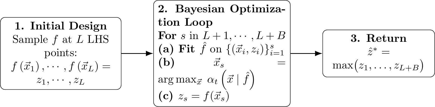
To initially fit the surrogate model, \(\hat{f}\), we first sample \(L\)=25 points using Latin Hypercube Sampling (LHS) (McKay et al. 1979), a space-filling design-of-experiments method. LHS divides each input dimension of the bounded parameter space (the “hypercube” defined by the physically plausible ranges of \(\vec{x} = (\chi, c, V_t)\)) into \(L\) equal-probability intervals and places exactly one sample in each interval, guaranteeing that the full extent of each parameter is well covered with far fewer points than a full grid. After this we use the max-value entropy search (MES) acquisition function \(\alpha_t\) (Wang and Jegelka 2017), which selects each new evaluation point \(\vec{x}\) to maximise the expected reduction in entropy about the value of the global maximum \(z^{*} = \max_{\vec{x}} f(\vec{x})\), balancing exploration of uncertain regions with exploitation of regions likely to be near the optimum; we use MES to sequentially select an additional \(B=25\) Bayesian optimization points to evaluate, refitting the surrogate model \(\hat{f}\) after each additional sample. This is shown as a flowchart in Figure 3.4.
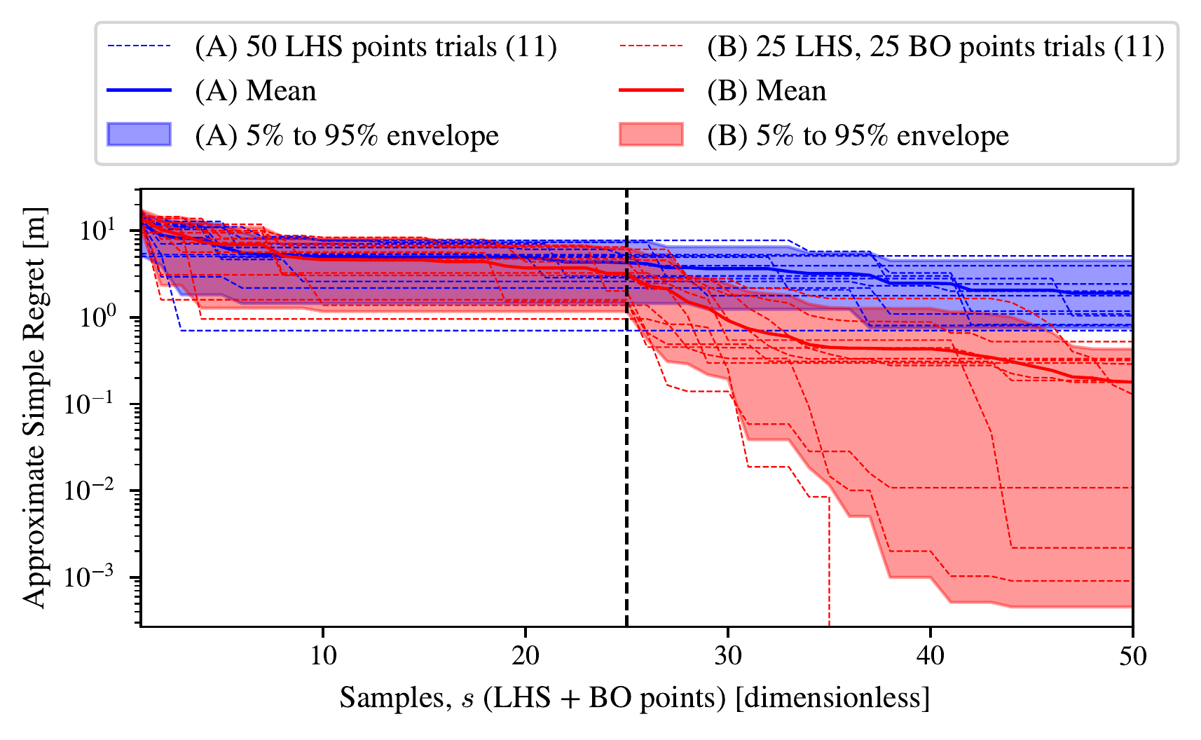
The number of initial points \(L\) and additional points \(B\) to select is chosen arbitrarily, although we show in Figure 3.5 that using the MES DAF leads to substantially better optima for one particular point than continuing to sample points using LHS. In strategy (A) we just use a Latin hypercube search (LHS) to fill the space with 50 samples (\(L=50\), \(B=0\)). In strategy (B) we first use 25 LHS samples and then 25 samples using the maximum value entropy search (MES) data acquisition function (\(L=25\), \(B=25\)). As defined, the two strategies are equivalent up until the 25th sample. To show the difference between the two strategies for optimization, in Figure 3.5 we plot the approximate simple regret, which we define as the difference between the current maximum observed storm surge, \(\max\left(\vec{z}^i_{1,\cdots,s}\right)\), up to that sample index \(s\) in the trial index \(i\) and the maximum over all \(n\) trials and all samples (the full budget), \(\max\left(\max\left(\vec{z}^1\right), \cdots \max\left(\vec{z}^n\right)\right)\), which serves as a proxy for the true global optimum, so that \[\begin{equation} \text{Approximate Simple Regret}_{si} = \max\left(\max\left(\vec{z}^1\right), \cdots \max\left(\vec{z}^n\right)\right) - \max\left(\vec{z}^i_{1,\cdots,s}\right). \end{equation}\](3.3)
This approximate simple regret is a measure of how much the maximum of the trials is behind the approximate global maximum, and is used in place of the simple regret (see e.g. D. Wang et al. (2022)). Each trial \(i\) uses a different random seed for the LHS design, so the initial points differ between trials; this allows us to estimate the variance of the optimisation strategy. As expected, the two strategies appear indistinguishable with the trials of the two experiments overlapping before the 25th sample (dashed line), because both select the same 25 LHS points. By 25 additional points (50 points total) then all trials of using Bayesian optimization with the MES DAF in strategy (B) outperform continuing with additional LHS space filling points in strategy (A). Therefore, this suggests that we can be confident that strategy (B) used for later experiments is superior to a simple LHS design, at least for this point on the coast, for finding a higher optima with equal computational resources. This does not show that strategy (B) is the optimal strategy, and it is possible that a different ratio of LHS to DAF samples, a different DAF (e.g. Expected Improvement as in Ide et al. (2024)), and an improved GP kernel (see e.g. Tazi et al. (2023)) could all improve the performance of the optimization strategy, where the best setting for each could depend on the point on the coast.
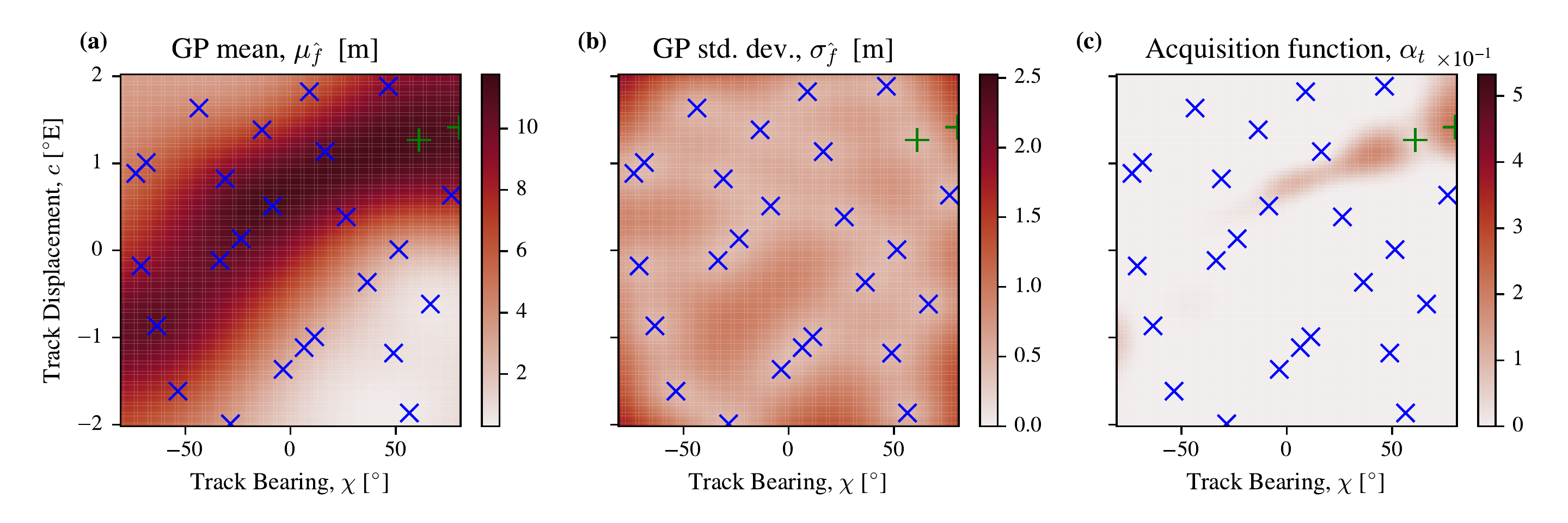
At the end of the Bayesian optimisation, the ADCIRC ensemble at each coastal point consists of \(L + B = 25 + 25 = 50\) simulations. An example of the Bayesian Optimization process (continuing to follow strategy (B), as in the rest of this paper) is shown in Figure 3.6, where, for clarity, we vary just the TC track’s bearing and displacement east and west of New Orleans. We use ADCIRC to compute the maximum storm surge height at the point in the mesh closest to New Orleans, and define this as the storm surge height. In all of the panels, we plot the initial 25 points/ADCIRC simulations selected through Latin Hypercube sampling as blue crosses (x), and show the three additional points selected by Bayesian optimization as green plusses (+). The LHS points are spread evenly across the parameter space for broad initial coverage, while the MES acquisition function selects additional points where the GP predicts high storm surge and uncertainty remains large, encoding the exploration–exploitation trade-off that concentrates subsequent samples near the likely optimum. Figure 3.6(a) shows the GP emulator’s mean, \(\mu_{\hat{f}}\left(\vec{x}\right)\), and Figure 3.6(b) shows the emulator’s standard deviation \(\sigma_{\hat{f}}\left(\vec{x}\right)\), after it has been fitted on all of the points sampled so far. In Figure 3.6(b) the standard deviation of the emulator is much lower around the points which have already been sampled. We can see that the emulator expects the highest maximum storm surge heights to be reached either at positive bearing and positive track displacement or negative bearing and negative track displacement, forming a band of higher values (Figure 3.6(a)). The two green points that have already been sampled are at positive bearing and positive track displacement, suggesting this end of the track-bearing ridge has the highest emulator values \(\hat{f}\). The MES DAF in Figure 3.6(c) is highest near the three additional points that have already been selected, so that the model will continue to explore this area of the parameter space for the next sample.
3.2.5 Fitting a Generalized Extreme Value Distribution
In the final part of the framework, we explore whether knowing the potential height can improve estimates of long return-period storm surges. Estimating rare events from data is fundamentally limited by sample size: a 50-year tide-gauge record contains at most 50 annual maxima, far too few to constrain 100- or 500-year return levels without strong distributional assumptions. Extreme value theory (EVT) provides the standard statistical framework for such extrapolation (Coles 2001). Under the block-maxima approach, the annual maximum storm surge at a given location is modelled as an independent draw from a Generalized Extreme Value (GEV) distribution, justified by the Fisher–Tippett–Gnedenko theorem (Fisher and Tippett 1928; Gnedenko 1943). Because no real observations are available with which to test return levels of hundreds of years, we instead conduct a set of idealised Monte Carlo simulations: we draw synthetic annual-maximum samples from a known GEV distribution and ask how well the fitting procedure recovers the true return levels, with and without knowledge of the upper bound.
If we consider the case where we have block-maxima observations (the maximum storm surge height recorded each year), then we would expect that we can model the dataset \(\vec{z}\) of \(N_s\) observations as samples from a Generalized Extreme Value (GEV) distribution (Coles 2001). If we assume the existence of a maximum \(z^{*}\) that the distribution should reach corresponding to the potential height, we can assume the distribution is of the Weibull class. For the case of the GEV distribution the probability density function is given by \[\begin{equation} \mathrm{GEV}\left(z; \alpha, \beta, \gamma\right) = \frac{1}{\beta}\left[1+\gamma\left(\frac{z-\alpha}{\beta}\right)\right]^{-1 - \frac{1}{\gamma}} \exp{\left\{-\left[1+\gamma\left(\frac{z-\alpha}{\beta}\right)\right]^{- \frac{1}{\gamma}}\right\}}, \end{equation}\](3.4) where \(z\) is the maximum height of the storm surge above the coast for a particular year, \(\alpha\) is the position parameter, \(\beta\) is the scale parameter, and \(\gamma\) is the shape parameter, which should be \(\gamma<0\) for the Weibull class distribution. We can then find the upper bound \(z^{*} =-\frac{\beta}{\gamma}+\alpha\).
In the case where we exactly know the upper bound ahead of time (case
I) this leaves us with two parameters to fit, \(\beta\) and \(\gamma\). If we do not know the upper bound
ahead of time (case II) and have to fit it, we have three parameters to
fit \(\alpha\), \(\beta\), and \(\gamma\). In both cases we can minimize the
negative log-likelihood of the dataset \(\vec{z}\) with respect to the parameters
using tensorflow with the Adam optimizer (Kingma 2014) for
1,000 optimization steps with a learning rate of 0.01, \(\beta_1=0.9\), \(\beta_2=0.99\), and \(\epsilon=10^{-6}\) which were the default
parameters.
To assess the recovery of the original distribution (i.e. the ability of the fitting procedure to recover the true underlying GEV parameters from a finite sample) with these two cases (I and II), we take \(N_s\) samples from a GEV distribution, and choose the parameters \(\alpha=2 \text{m}\), \(\beta=1 \text{m}\), and \(\gamma=-0.2\), and therefore \(z^{*}=7 \text{m}\). To estimate the uncertainty in the model parameters we resample the dataset \(N_r=600\) times for each setting and refit both cases each time. This was chosen empirically, as we found \(N_r=600\) to be large enough to reliably estimate confidence intervals. In order to focus on metrics of interest for risk professionals we focus on the 1 in 100 year (0.01% exceedance probability per year) and 1 in 500 year (0.002% exceedance probability per year) return values calculated from the fitted distributions. For each case using these \(N_r=600\) estimates, we calculate the mean and the 5% and 95% for both return values.
Because of calculation error, and simplifications made in each part of the Potential Height framework, we will not know the upper bound exactly. We can make case I more realistic by adding some Gaussian noise to the true upper bound \(z^{*}\) so that the ‘calculated’ upper bound is \(\hat{z}^{*}=\mathcal{N}\left(z^{*}, \sigma_{z^{*}}\right)\) where \({\sigma}_{\hat{z}^{*}}\) is the standard deviation in the ‘calculated’ upper bound that we can vary. Data points larger than the ‘calculated’ upper bound would have zero likelihood in case I, but to mitigate this we assume that if there is a higher value in the sampled dataset, \(\vec{z}\), we replace the ‘calculated’ upper bound with the ‘empirical’ upper bound, \(\hat{z}^{*\prime} = \max\left(\hat{z}^{*}, \max\left(\vec{z}\right)\right)\). We can then use this adjusted upper bound \(\hat{z}^{*\prime}\) in case I, sampling a new \(\hat{z}^{*}\) each time we resample the dataset \(\vec{z}\), \(N_r=600\) times. These adjustments do not affect case II.
3.3 Results
| Parameter | Symbol | Value |
|---|---|---|
| ADCIRC storm surge model | ||
| Mesh | EC95c | 31,435 nodes; 58,369 elements |
| Timestep | \(\Delta t\) | 5 s |
| Simulation duration | 7 days (1 day ramp) | |
| Forcing grid (static) | \(\frac{1}{8}^{\circ}\) | |
| Forcing grid (moving) | \(\frac{1}{80}^{\circ}\) | |
| TC track parameters | ||
| Track bearing | \(\chi\) | \((-80^{\circ},\; 80^{\circ})\) |
| East–west displacement | \(c\) | \((-2^{\circ}\text{E},\; 2^{\circ}\text{E})\) |
| Translation speed | \(V_t\) | \((0,\; 15)\) m s\(^{-1}\) |
| Bayesian optimisation | ||
| Initial LHS points | \(L\) | 25 |
| BO (MES) points | \(B\) | 25 |
| Total ensemble size | \(L+B\) | 50 per coastal point |
| GP kernel | Matérn 5/2 | |
| Acquisition function | \(\alpha_t\) | MES (Wang and Jegelka 2017) |
In this section, we implement our framework to calculate the potential height of a storm surge at a point along the coast of New Orleans. We investigate how the maximum storm surge changes as we vary the parameters of a TC. We choose to use the years 2025 to represent the present day climate conditions and 2097, which produces a substantially larger potential intensity and potential size, to represent climate conditions at the end of the century. We use the SSP-585 emissions scenario CESM2-r10i1p1f1 ensemble member August mean to calculate the potential size and potential intensity of the storm. We assume that the TC reaches these potentials, i.e maximum intensity and size that are physically plausible, given the monthly average meteorological conditions. We implement the TC profile of Chavas et al. (2015) to model the respective wind field, and use it to force ADCIRC, varying track displacement, angle, and velocity (\(c,\; \chi,\; V_t\)).
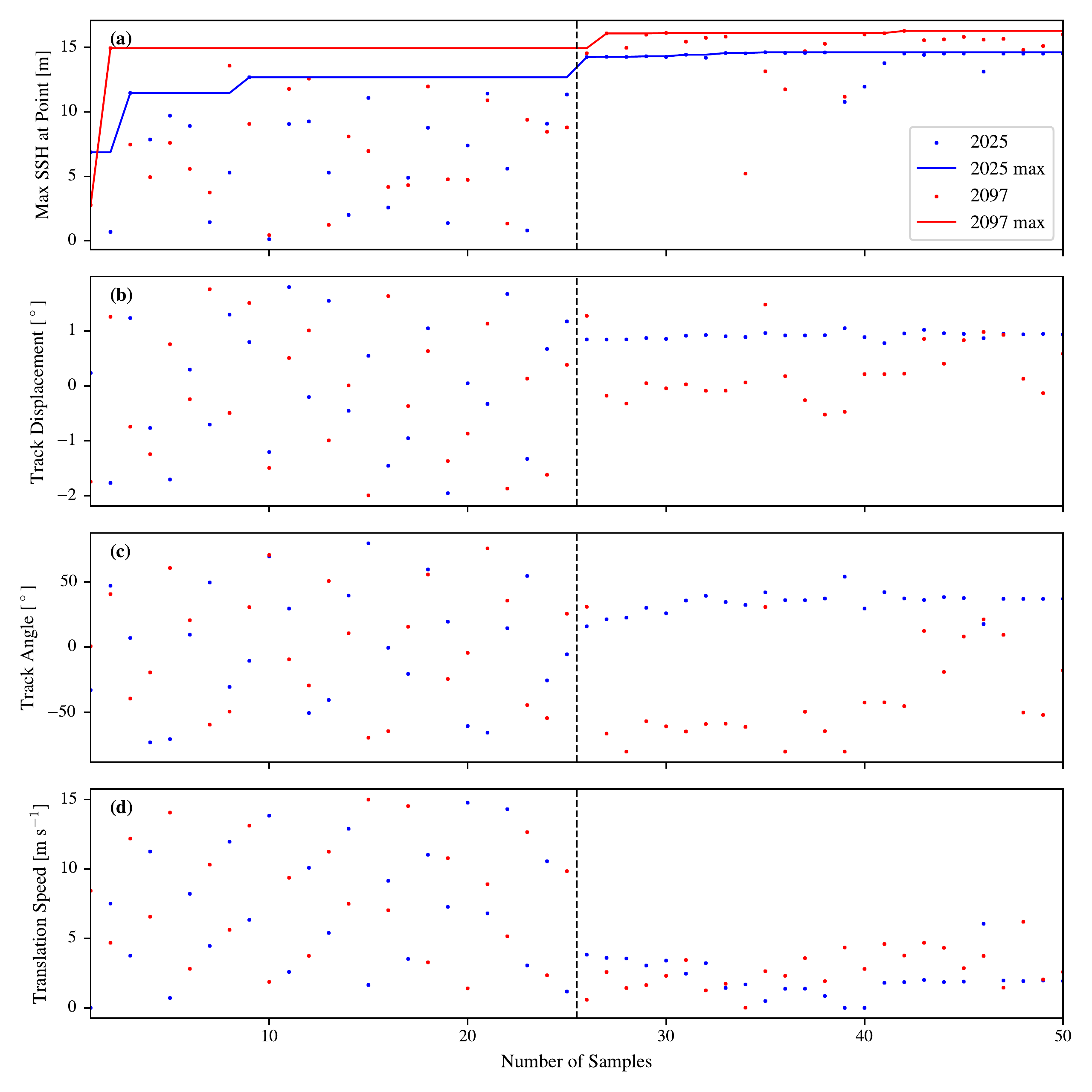
We choose to use the triangular vertex in the ADCIRC mesh closest to the center of New Orleans for our analysis. We first perform 25 ADCIRC simulations using a Latin hypercube to sample the full range of TC parameters. These data points including the simulated surges are used to create an initial fit for the emulator. We then use the MES acquisition function to optimally sample another set of TC parameters, and perform another 25 ADCIRC simulations. Figure 3.7 shows the results of this process, where panels (b-d) describe the TC characteristics used to force the \(i\)-th ADCIRC simulation. Figure 3.7(a) shows the maximum storm surge height produced from each sample, and the largest heights produced from the full optimization procedure is denoted by the solid line. For this example location, the maximum storm surge attained by this optimization is 0.87 m higher in 2097 than in 2025. There is some uncertainty associated with the optimization procedure, as it is possible that the function has not found the global optima in each case. In Figure 3.7(b)-(d) we can see that the optimal TC track parameters are quite close to one another for the two years, as we might expect. TC track displacement is measured east and west of the observation point.
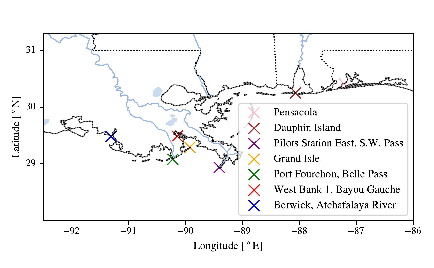
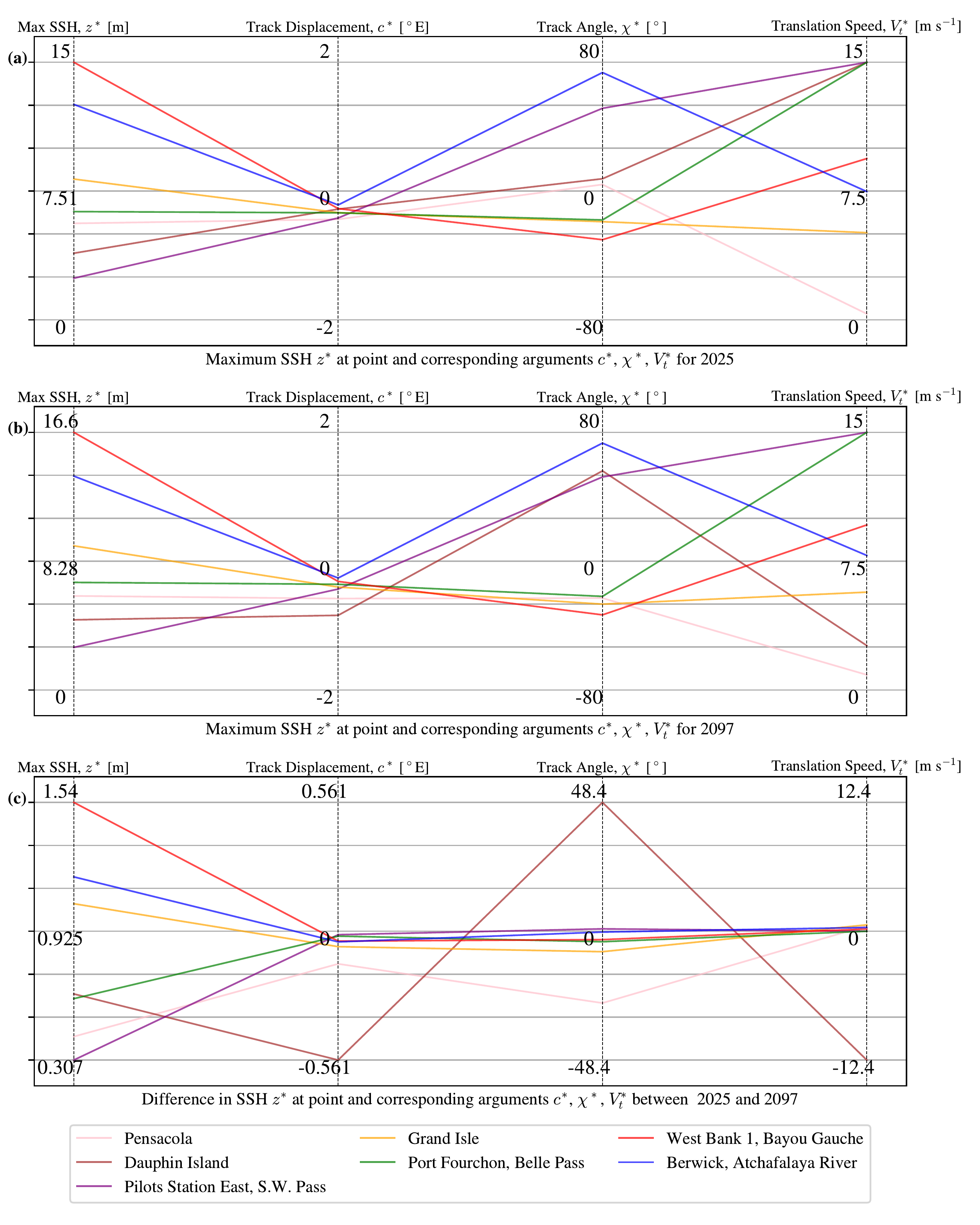
In Figure 3.9 we show the results from conducting two sets of Bayesian optimisation experiments. We use the CLE15 wind and pressure profiles with the potential size and intensity calculated for August 2025 and August 2097 using the CESM2-r4i1p1f1 SSP585 ensemble member. The locations of the points are shown in Figure 3.8. The potential height values found for 2097 in (b) are uniformly higher than those for 2025 in (a) as shown in panel (c), as expected because the potential height and potential intensity are higher. In each experiment for all points, the optimal displacement ends up being slightly to the west of the observation point, which would likely correspond to the TC’s top right corner passing over the points, which agrees with our expectations. The optimal parameters are in general similar between the two years for both locations for every point (panel c), apart from for the point near Dauphin Island, where the track displacement, track angle, and translation speed are all drastically different between the two, despite it following the general trend of an increased Max SSH. There are several possible explanations for this behaviour. First, the storm surge response surface at Dauphin Island may be multimodal, with multiple distinct TC track configurations producing similarly high surges; a small shift in potential size or intensity between the two climate periods could then tip the global optimum from one mode to another. Second, it is possible that the Bayesian optimization has converged to different local maxima in the two periods, a known limitation of surrogate-based optimization with a finite evaluation budget. Third, the change in potential size and intensity between 2025 and 2097 could genuinely shift the optimal track geometry at this location, for example because Dauphin Island’s exposed coastal geometry makes the surge response more sensitive to the angle of approach than the more sheltered sites. Without additional experiments, such as running a denser grid search or repeating the optimization with more trials, it is not possible to conclusively distinguish between these explanations, and the Dauphin Island result should therefore be interpreted with caution. For the other points, the significant change is the movement of the track displacement slightly westward (negatively in displacement), which could correspond to an increase in the potential size \(r_a\) and radius of maximum winds \(r_{\mathrm{max}}\) between the two years tested. The two headlands of Port Fourchon and Pilots Station East both have optima in both years with the maximum allowed translation speed of 15 m s\(^{-1}\) whereas the more enclosed points at Pensacola, West Bank 1, and Berwick all have much slower optimal translation speeds (1 m s\(^{-1}\), 7.5 m s\(^{-1}\), & 2 m s\(^{-1}\) respectively). This is compatible with Lockwood et al. (2022)’s finding that open coastal points have higher storm surge heights at higher TC translation speeds, whereas semi-enclosed coastal points have lower storm surge heights at higher TC translation speeds. The average maximum SSH (potential height) found for the set of points increases by 0.8 m or 11% between 2025 and 2097, equivalent to an average rise in potential height of around 1 cm yr\(^{-1}\).
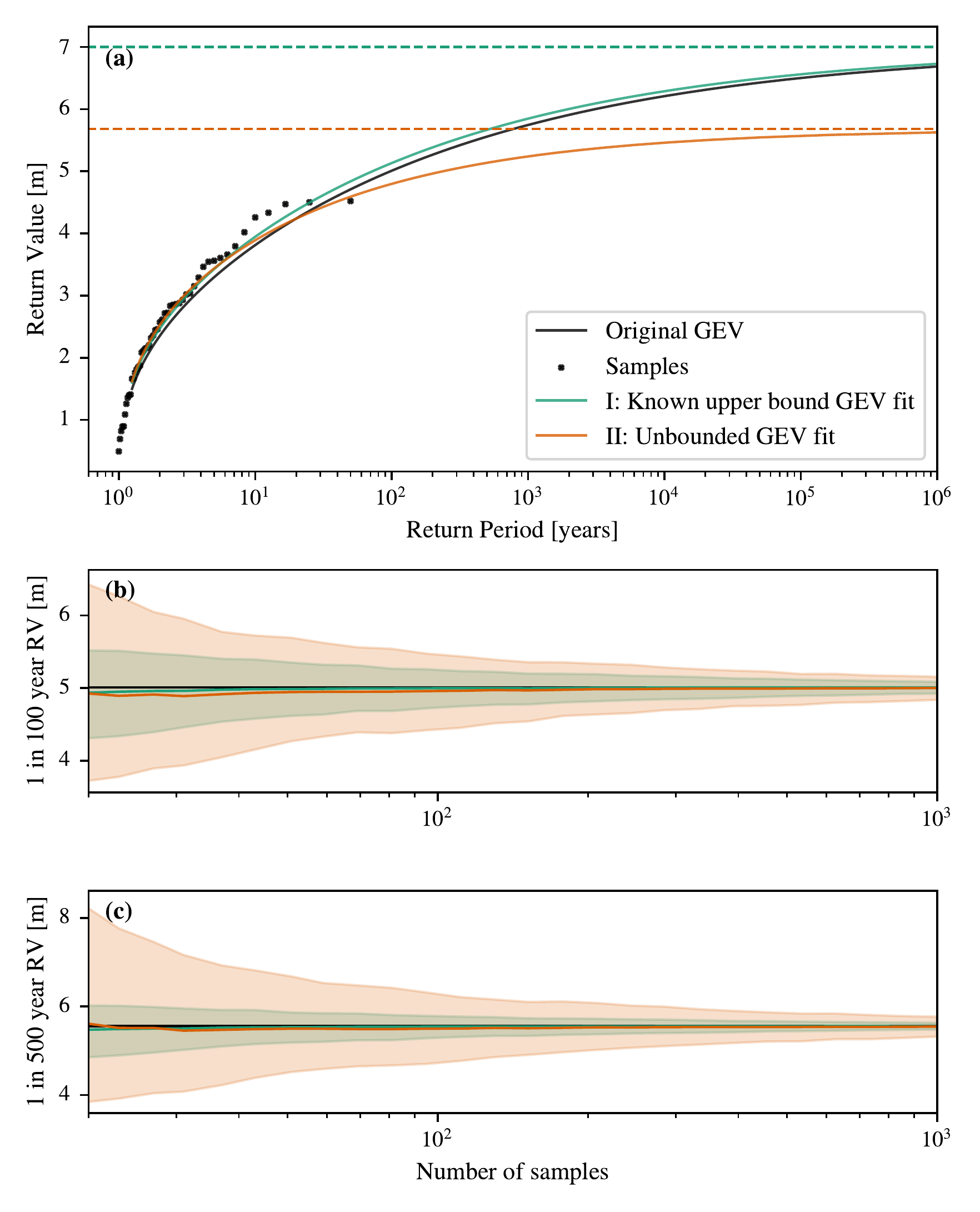
To highlight the usefulness of these estimates, we run a statistical simulation to investigate the impact of implementing a determined upper bound on the sampling uncertainty given \(N_s\) years of block maxima observations at the point of interest. To do this, we fit the generalized extreme value distribution both with and without assuming the upper bound we have computed, i.e. the worst case storm surge height. We assume that the maximum storm surge height observed each year is sampled from the “true" generalized extreme value (GEV) distribution. In Figure 3.10(a) a sample of 50 data points (\(N_s=50\)) from the assumed GEV (\(\alpha=2 \text{ m}, \beta=1 \text{ m}, \gamma=-0.2\)) are denoted by the black dots. Their return period \(p\) is estimated as \(p=(N_s+1)/(r)\) where \(N_s\) is the number of yearly maxima sampled and \(r\) is the rank (order) of the sample, i.e. \(\left\{ 1, ..., N_s \right\}\) in descending order. For the GEV distribution itself, the return period of the distributions \(p\) for a return value \(v\) is calculated as \(p =1/(1-F(v))\) where \(F\) is the cumulative distribution of the fitted distribution. We fit a GEV to this set of sampled data points, assuming the upper bound (\(z^{*}=7\) m) is known (I, green) or unknown (II, orange). We see that (I) is very close to the true distribution (black), whereas (II) is substantially different. The dashed lines show the upper bound of the fitted distribution for the case where the upper bound was known ahead of time (green) and the case where it was not (orange). For this example the fit for case I (green) where the upper bound was known ahead of time is much closer to the true distribution (black line) than case II (orange), where the upper bound was not known. In particular, case II significantly underpredicts the upper bound compared to the true value, whereas case I is guaranteed to have the same upper bound.
To explore this effect more systemically, we repeat the implementation \(N_r=600\) times for various numbers of samples (\(N_s\)).
The number of samples taken (\(N_s\)) is varied between \(N_{s\; \text{min}}=15\) and \(N_{s\;\text{max}}=1000\), and for each number of samples the original GEV is resampled \(N_r=600\) times with different random seeds. The distributions are refitted for each of the \(N_r=600\) resamples, and the 1 in 100 year and 1 in 500 year return values of that fit are calculated. From the \(N_r=600\) resamples for each sample size \(N_s\) we calculate the mean fit prediction over the resamples (solid lines) and the 5% to 95% envelope (colored envelopes). This is shown in Figure 3.10(b)&(c), where we can see that a mean prediction across the resamples in either case is very close to the true value (black line) for both the case where the upper bound is known (green line), and unknown (orange line) for the 1 in 100 and 1 in 500 year return values independent of the number of samples taken, \(N_s\). However, as expected, the confidence envelope for both substantially declines as the number of samples, \(N_s\), is increased. For both return levels, the effect of knowing the upper bound (green envelope) substantially reduces the 5th-95th percentile envelopes when compared to not knowing the upper bound (orange envelope). This effect is more substantial at the 1 in 500 year return level than the 1 in 100 year return level, and for example at \(N_s=51\), the 5%–95% range is reduced \(1.98\times\) for the 1 in 100 year return value, and \(3.18\times\) for the 1 in 500 year value.
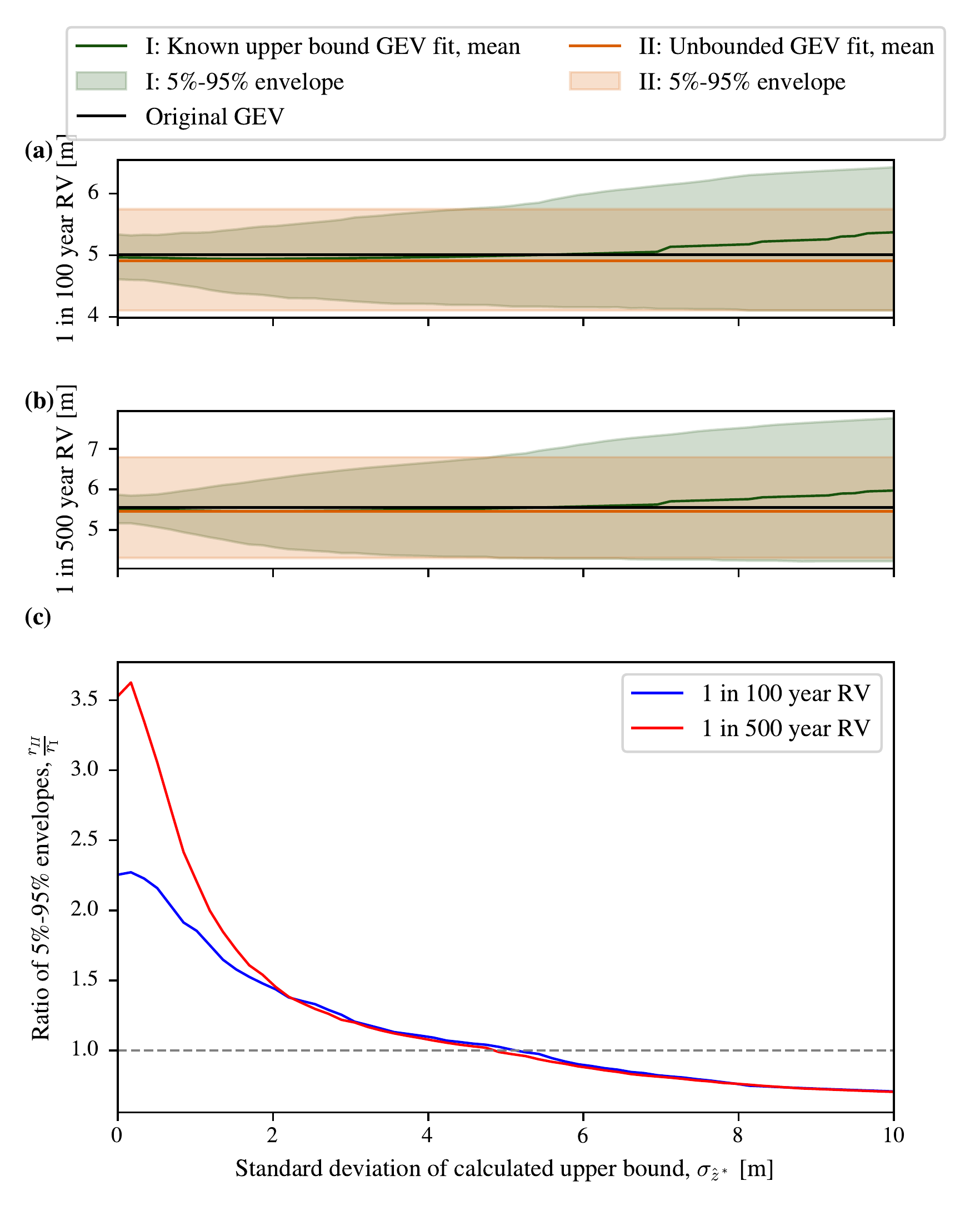
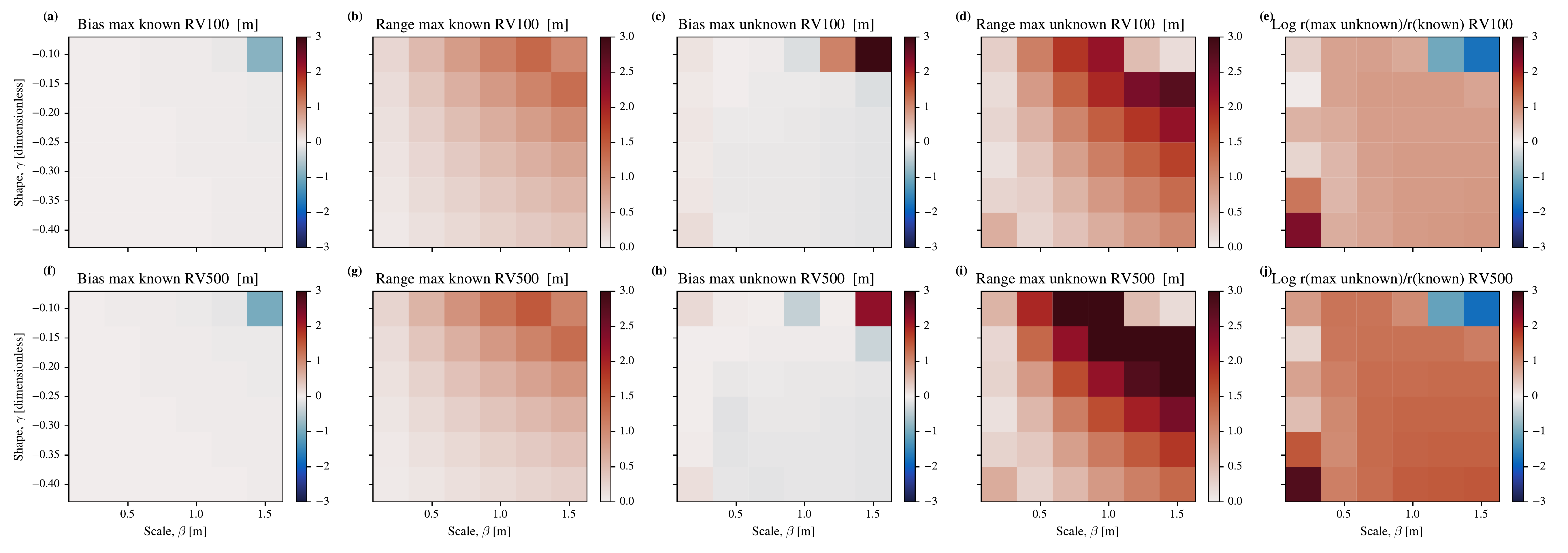
To investigate whether the results still hold when we vary the uncertainty in the ‘calculated’ upper bound, we vary the assumed Gaussian noise level while keeping the number of samples at \(N_s= 50\) in Figure 3.11. Figures Figure 3.11 (a) & (b) show the mean and the 5%-95% envelopes for the 1 in 100 and 1 in 500 year return values (RV) for fitting methods (I) and (II), where we change the standard deviation in the calculated upper bound \(\sigma_{\hat{z}^*}\) for method (I). As shown in the two panels, an estimate of the upper bound (I) reduces the bias in the mean estimate, and leads to a smaller 5%–95% envelope, until it is very large \(\sigma_{\hat{z}^*}>5\text{ m}\). As \(\sigma_{\hat{z}^*}\) progresses from 0 m to 5 m (where the scale is 1 m), the range of (I) approaches (II). To show this quantitatively, in Figure 3.11(c) we can see that the ratio between the 5%-95% confidence envelopes begins larger for the 1 in 500 year events than the 1 in 100 year events, as knowing the upper bound has a larger effect on our estimation of longer return period return values as before. Both reach 1.0 at \(\sigma_{\hat{z}^*}\approx 5 \text{ m}\) as the standard deviation in the calculated upper bound increases and the information becomes less informative. This might be surprising because it suggests that knowing the upper bound in this set up, even with this large standard deviation, improves the return value estimate. This could be because if the calculated upper bound is too low, then it is likely to be replaced by the maximum of the samples, and if it is too high, then the shape and scale parameters can change to compensate and achieve good long period RV, but this should be studied further. When we go beyond this, \(\sigma_{\hat{z}^*}>5\text{ m}\), then the range of method (I) is greater than method (II) as shown in Figure 3.11(c). We can also see that the mean prediction in Figure 3.11 (a) & (b) begins to increase sharply at \(\sigma_{\hat{z}^*}>7\text{ m}\), suggesting that at this point the unrealistically high upper bounds assumed do have a negative impact. The bias is positive because if an unrealistically low upper bound is sampled for \(\hat{z}^*\) then it is likely to be replaced with the maximum of the observations \(\mathrm{max}\left(\vec{z}\right)\).
3.4 Discussion
3.4.1 Summary of Findings
Through our initial results we have shown the implications of finding the maximum potential height of a TC storm surge and how it may increase due to climate change. Key findings of our work include: (i) that Bayesian optimization can be used to more efficiently find the maximum storm surge height produced by a TC with a variable trajectory, (ii) that the combined increase in potential size and potential intensity leads to a mean increase of 8% in the maximum storm surge height at seven points along the coast of New Orleans over the 21st century, and (iii) that in idealized simulations, knowledge of the upper bound of the potential storm surge height can substantially reduce the uncertainty in the 1 in 100 and 1 in 500 year return values, even if there is uncertainty in the upper bound. It is our hope that this work will provide foundational bases for further work on the topic.
3.4.2 Potential Size
To our knowledge, this is the first time that potential size has been calculated for a specific geographic region or as a time-varying characteristic. It is also the first time we have seen it utilized in constraining estimates of storm surge risk. By driving the ADCIRC model with the CLE15 profile, and assuming an isothermal inflow when integrating to find the pressure profile, we made our forcing method as consistent with the potential size calculation as possible. Our implementation allows us to show that the potential size is expected to increase in the future and is highly correlated to the sea surface temperature. We found that the potential size increases by around 2.3 km per year in the SSP585 ensemble members that we investigated. Combined with the increase in potential intensity, this leads to a mean increase in the calculated potential height of 0.8 m (11%) across seven coastal points near New Orleans between August 2025 and August 2097.
Here we have used just a single CMIP6 model member and a single high-emission scenario to exemplify the use of our framework for investigating possible effects of climate change on the storm surge hazard. SSP-585 is now considered to be a less likely emissions scenario (e.g. Huard et al. (2022)), and so more likely results for risk quantification can be explored by using intermediate scenarios. It would be worthwhile to compare the results produced by using different CMIP6 models and scenarios to explore more systematically whether different ensemble members exhibit different relationships to potential intensity and size.
We also use monthly averages to calculate potential intensity and size, but potential intensity and size could vary significantly within months. For example, marine heat waves could increase the potential intensity of TCs. An alternative approach is to consider a particular percentile of potential intensity, as was done in Mori et al. (2022), to consider, for example, the 1 in 10 year potential intensity, and work out the corresponding storm surge that this would produce.
There are some key issues that might affect our estimates of potential size and intensity. First, the potential size measure does not include a number of important processes, such as the dissipation of energy through eddy shedding (D. Wang et al. 2022). As noted by D. Wang et al. (2022), their derivation also excludes some time-varying effects, such as the ventilation of colder water to the surface, which is also true for potential intensity as calculated (Bister and Emanuel 2002). Additionally, it relies on a number of tuneable parameters, such as the dissipation rate, \(w_{\mathrm{cool}}\), the efficiency relative to the Carnot engine, \(\eta_\mathrm{rel. carnot}\), and the supergradient factor, \(\gamma_{\mathrm{sg}}\). As these values may have been tuned to match the numerical simulations of azimuthally symmetric TCs in D. Wang et al. (2022), the potential size has some degree of subjectivity. D. Wang et al. (2022) compares the calculated potential size against numerical simulations of TCs, but they do not compare the measure against observations. Comparing TC sizes recorded in terms of \(r_{\mathrm{max}}\) from the International Best Track Archive for Climate Stewardship (IBTrACS, Knapp et al. (2018)) to the potential sizes calculated using ERA5 data (Hersbach et al. 2020) would support verification of the potential size model, and allow us to assess the distribution of sizes as a fraction of potential size that has been observed (similar to Emanuel (2000)).
Finally, there may be broader theoretical inconsistencies made in the derivations of potential intensity and size that we have not explored here. First, though Emanuel (1986)’s potential intensity is well-established and relatively well accepted (Rousseau-Rizzi et al. 2021), Makarieva and Nefiodov (2023) suggests that the model has an internal thermodynamic inconsistency. There are also a number of assumptions made in the Chavas et al. (2015) profile that join together the analytic solutions from Emanuel and Rotunno (2011) and Emanuel (2004), both of which were analytically derived. D. Wang et al. (2022) and Wang et al. (2023) use a more detailed Carnot engine to calculate the pressure drop to the radius of maximum wind than Emanuel (1986), and so recalculating the potential intensity \(V_{p}\) in a way that is congruent with this calculation is worth further exploration.
3.4.3 Bayesian optimization
We have shown that Bayesian optimization can be used to find the potential height at different points along the coast, for two different years, showing the increase in potential height between them. For the set of seven points near New Orleans that were chosen, the average increase in calculated potential height was 0.8 m (11%) between August 2025 and August 2097.
The only source of uncertainty accounted for within the Bayesian optimization is that of the GP surrogate model: the MES acquisition function uses the GP’s predictive distribution, both its mean and variance, to decide where to sample next. However, we do not propagate upstream uncertainties into the optimization. In particular, the potential intensity and potential size are treated as fixed inputs derived from a single climate model ensemble member and month, without accounting for uncertainty in the climate fields, the physical model approximations (e.g. the Carnot engine assumptions, tuneable parameters in the potential size calculation), or the TC wind profile. As a result, the GP surrogate’s uncertainty reflects only how well the emulator has learned the mapping from TC track parameters to storm surge height, and does not capture the full uncertainty in the final potential height estimate. Propagating these upstream uncertainties, for example by sampling over multiple climate ensemble members, months, or parameter settings, is an important direction for future work.
In Figure 3.5 we show that our framework improves upon randomly selecting points in terms of minimizing simple regret. We used the MES data acquisition function of Wang and Jegelka (2017) to optimize the trajectory of a TC, which we expected to outperform the expected improvement acquisition function used in Ide et al. (2024). However, we have not compared our strategy against any other data acquisition functions, or verified that the strategy is superior for all the points along the coast. Bayesian optimization is also dependent on the performance of the emulator in capturing the relationship between the variables in the modelled space, and so adapting the kernel to be more appropriate to the problem (as in Tazi et al. (2023)), could lead to the strategy minimizing regret more effectively.
3.4.4 Statistical simulation
We use statistical simulation to investigate the utility of knowing the upper bound in improving the estimation of return values, based on samples taken from a GEV distribution. First, we investigate the effect of varying the sample size \(N_s\) on our estimates of the return values (in Figure 3.10), and find that knowing the true upper bound \(z^{*}\) improves the estimate of the return values, especially for smaller sample sizes and for the longer return period. Secondly, we assume some Gaussian error in the upper bound to investigate what would happen if we did not know this upper bound exactly, keeping \(N_s=50\) (Figure 3.11). We find that the uncertainty is improved with a moderate error (\(\sigma_{\hat{z}^*} \approx 1 \text{ m}\)) in the potential height of the storm surge, so we could expect it to improve relevant risk estimates, and only if it is extremely imprecise (e.g. \(\sigma_{\hat{z}^*}> 5 \text{ m}\)) would it reduce the quality of risk estimates. For both of these statistical simulations, we do not vary the values of \(\beta\) and \(\gamma\), but we expect (based on Figure 3.17) in Section Section 3.8, that our findings will also generalize to these parameters if they were varied for both experiments. Through these results, we have shown that calculating the potential height could usefully augment observations even with realistic calculation uncertainty.
Nonetheless, a number of caveats and unexplored questions remain. None of these simulations make use of real observations. As such, we have not fully explored the practical implications of applying this technique for different points on the coast or evaluating the change in estimated risk. Additionally, in our work we maximized the log-likelihood of the GEV parameter values given the data samples for simplicity. However, Jewson et al. (2025) show that doing so would lead to a negative bias where return periods are exceeded more often than would be expected, and that it would be better to use calibrating priors. Therefore, it is worth exploring whether the effects we see in these statistical experiments would still hold if we use a more advanced set of statistical assumptions. We have still assumed that the observations are i.i.d. and therefore ignore non-stationarity in the observations created by climate change.
3.4.5 Storm surge model improvements
To calculate the potential height of the storm surge we used an implementation of the ADCIRC model. Our implementation does not include all of the processes involved in creating the highest potential extreme water height along the coast. Specifically, we have excluded the effects of tides (including tide-surge interaction), wave run up and set-up, and sea level rise. To estimate the potential total water height that could be generated at a point along the coast, these processes should be included. Future studies can include tides in the ADCIRC model simulations, which can be optimized over by changing the time of impact in the simulation of the TC around the spring tide. The effects of waves can be included by using the ADCIRC’s popular coupling with the SWAN wave model (Booij et al. 1999), though this will add significant computational cost. Sea level rise can be included by adding a constant offset of additional water height to the existing ADCIRC simulation, taken from the same CMIP6 scenarios for self-consistency. Finally, Chaigneau et al. (2024) showed that using the baroclinic NEMO model improves the accuracy of simulated storm surge heights in areas such as on the Southeastern Florida Peninsula. Future research could use this model in place of the (barotropic) ADCIRC model, however this also comes with increased computational cost (more than 100 times).
In additional to climate change, the shape and position of the coastline will also change over the next 100 years, likely affecting the vulnerability of different communities to storm surges. For example, many coastal areas are undergoing subsidence (e.g. Nicholls et al. (2021)). Representing this in the ADCIRC model would necessitate changing the computational mesh. Different projections of the morphology of the coastline as well as the resulting dynamic sea level rise could be incorporated in the model in future studies.
3.4.6 Generalizations of this framework
The framework we have developed can be extended to any coastline and potentially to other environmental hazards such as extreme rainfall flooding, e.g. if comparable limits for rainfall were suggested. Here, we have focused on the US Gulf of Mexico and the New Orleans area in particular, but we could extend this work to more areas, such as East Asia. Indeed, the areas of the largest growth in economic exposure are expected in East, South East, and South Asia (e.g. for the Pearl River Delta, Deng et al. (2022)), due to population growth and economic growth in the coastal regions of these areas.
Both the total height of the water and the duration of its elevation above a certain level can have an impact on the damage done to a coastal community, as these provide more time for flood defences to fail, for flood water to propagate inland, and for water from pluvial and river sources to compound the flooding. While it may be much more difficult to construct physical bounds for TC rainfall, and for the pre-existing river levels that respond to that rainfall, it is worth considering optimization of a more combined measure that represents the damage done to the coastline such as that described in e.g. Zhang et al. (2000). Beyond the surge height itself, a natural next step is to connect the potential height output to a downstream impact or damage model that translates surge exposure into casualties, displacement, or economic losses. Studies such as Wing et al. (2022) have documented how flood risk and its impacts are distributed inequitably across communities, and the potential height framework developed here could serve as a physically grounded upper-bound input to such damage models, helping to characterise worst-case risk under present and future climates. Developing this link is beyond the scope of the current Chapter, which focuses on finding the potential height, but represents a clear and important extension.
3.5 Conclusion
We have seen that Bayesian optimisation can be used to efficiently relate the potential intensity and size of a TC to the corresponding maximum potential height of a storm surge at a point along the coast. Both potential intensity and size generally increase assuming projected climate change scenarios, and we are able to use the developed framework to estimate the corresponding increase in the potential height of associated storm surges. We have shown that knowledge of the maximum potential storm surge height can effectively reduce the uncertainty in return periods important for practical applications. However, we do not make use of data produced by nearby coastal points or different forcing scenarios, and this framework could be usefully extended by doing so. Further, we do not fully explore bias correction of climate data, which is important to understanding how TC potential size, intensity, and storm surge height change over time. Additionally, the ADCIRC grid used here (EC95c) is relatively coarse; a higher-resolution mesh would better resolve nearshore processes, complex coastal geometry, and localised surge features, and could change the estimated potential height at some locations, particularly semi-enclosed or shallow sites, so investigating the sensitivity to mesh resolution is an important direction for future work. We have developed our framework and made it available as a set of open-source Python packages, hopefully enabling the wider community to easily build upon this work. In the future, we hope this framework can be used to provide more robust and accurate risk estimation for different areas of the world.
Acknowledgements
Thank you to Tom Andersson (Google DeepMind), David Cross (JBA Risk Management), and Gordon Woo (Moody’s Risk Management Solutions) for helpful conversations on this topic.
ST is supported by studentship 2413578 from the UKRI Centre for Doctoral Training in Application of Artificial Intelligence to the Study of Environmental Risks (grant no. EP/S022961/1).
Conflict of interest
The authors declare no conflict(s) of interest.
Data availability statement
The GEV simulation data plotted was lightweight so has been added to the code repository (Thomas 2025b). The raw CMIP6 data is easily available from the Pangeo catalogue (Pangeo 2022).
Open source software
The main code to produce the figures for this paper is available at
https://github.com/sdat2/worstsurge (Thomas 2025b), with
ReadTheDocs documentation at https://worstsurge.readthedocs.io/en/latest/MAIN_README.html,
and builds on some utility scripts in the sithom package
(Thomas
2024). Initial exploration in ADCIRC emulation was performed in
Thomas (2025a).
Bayesian optimization is provided by the trieste package
(Picheny et al. 2023) which uses
gpflow (Matthews et al.
2017) and tensorflow (Abadi et al. 2015).
ADCIRC v55 (Pringle et al. 2021) is publicly
available at https://github.com/adcirc/adcirc, and our slightly
modified copy for the Archer2 HPC is available at https://github.com/sdat2/adcirc-v55.02 with our
compilation settings. The CLE15 TC profile of (Chavas et al. 2015) was
calculated using their original matlab implementation (Chavas 2022), but
using octave (Eaton et al. 2020) for accessibility.
3.6 Appendix: TC potential intensity and potential size details
Figure 3.12 shows how the potential size is calculated from the environmental variables taken from the CMIP6 model member. The key inputs to first calculate the potential intensity using tcPyPI (Gilford 2021) are the sea surface temperature of the water (from the ocean monthly average table, Omon, TS, \(T_s\)), the mean sea level pressure (MSL, \(p_s\)), air temperature column (TA, \(T_a\left(p\right)\)) and specific humidity (Q, \(q\left(p\right)\)) column (all from the atmospheric monthly average table, Amon). The outflow temperature \(T_0\) and level \(OTL\) is calculated by following a moist adiabat from the sea surface to the point of intersection with the observed atmospheric profile. tcPyPI then calculates the potential intensity, \(V_p\), following Bister and Emanuel (2002) as, \[\begin{equation} \left(V_{p}\right)^2 = \frac{T_s}{T_0}\frac{C_k}{C_D} \left(\mathrm{CAPE}^{*} - \mathrm{CAPE}\right)\mid_{\mathrm{RMW}}, \end{equation}\](3.5) where \(V_{p}\) is the potential intensity at the gradient wind level, \(\mathrm{CAPE}^{*}\) is the convective available potential energy of saturated air lifted from the sea surface to the outflow level, and \(\mathrm{CAPE}_{\mathrm{env}}\) is the convective potential energy of the environment. The convective available potential energy is conventionally defined as the work done per unit mass by the buoyancy force acting on an air parcel from its level of free convection \(h_{\mathrm{LFC}}\) to its level of neutral buoyancy \(h_{\mathrm{LNB}}\), \[\begin{equation} \mathrm{CAPE} = {\int_{h_{\mathrm{LFC}}}^{h_{\mathrm{LNB}}}} B dh = g {\int_{h_{\mathrm{LFC}}}^{h_{\mathrm{LNB}}}} \frac{\rho_{e} - \rho_{p}}{\rho_{e}}dh, \end{equation}\](3.6) where \(B\) is the Buoyancy force per unit mass, \(\rho_{p}\) is the density of the parcel lifted to \(h\) and \(\rho_{e}\) is the density of the environment at \(h\), We assume that the air is lifted on a moist adiabat, exchanging no entropy with the surrounding air during ascent. When calculating the potential intensity, the ratio of the surface enthalpy exchange to momentum exchange coefficient \(\frac{C_k}{C_D}\) is assumed to be 0.9. Therefore, calling the tcPyPI package ends up looking like, \[\begin{equation} \mathrm{tcPyPI}\left(T_s, p_{\mathrm{msl}}, T_a\left(p\right), q\left(p\right), \frac{C_k}{C_D}\right) = \left(V_{p}, P_{\mathrm{min}}, T_{0}, \text{OTL}\right), \end{equation}\](3.7) where \(T_s\) is the sea surface temperature, \(p_{\mathrm{msl}}\) is the sea level pressure, \(T_a\left(p\right)\) is the air temperature profile, and \(q\left(p\right)\) is the specific humidity profile. The minimum central pressure \(P_{\mathrm{min}}\) is also calculated, but not used to calculate the potential size \(r_a\) or determine the final TC to force the ADCIRC model. When calling tcPyPI we do not reduce the potential intensity (feeding \(V_{\mathrm{reduc}}=1\)) so that \(V_p\) corresponds to the windspeed above the boundary layer rather than the 10m wind to be consistent with the CLE15 model. We later reduce the CLE15 wind profile by \(V_{\mathrm{reduc}}=0.8\) as detailed in Section Section 3.7 before it is applied to ADCIRC which is the standard value in tcPyPI (Gilford 2021).
To then go from potential intensity to potential size, we use the procedure described in D. Wang et al. (2022) with some additional assumptions, where we find the outer radius \(r_a\) that produces the same pressure at the point of maximum winds \(p_m\) with D. Wang et al. (2022)’s Carnot cycle (W22) and the Chavas et al. (2015) TC radial atmospheric profile (CLE15).
We first assume that the maximum windspeed used in the W22 Carnot engine \(V_{\mathrm{max\; W22}}\) is a supergradient constant \(\gamma_{\mathrm{sg}}=1.2\) above the maximum gradient wind assumed for the CLE15 model \(V_{\mathrm{gm}}\), which we further assume is the potential intensity calculated by the tcPyPI package, \(V_{p}\) so that \[\begin{equation} V_{\mathrm{max\; W22}} = \gamma_{\mathrm{sg}}V_{\mathrm{gm}} = \gamma_{\mathrm{sg}}V_{p}, \end{equation}\](3.8) as in D. Wang et al. (2022) Equation 23. This is allowed in the calculation of potential size (see D. Wang et al. (2022) sections 2b and 2c) but it is not the only possibility. This also introduces some inconsistency between assuming one Carnot cycle from Emanuel (1986) to calculate \(V_{p}\) and a more complex Carnot cycle to calculate the thermodynamic constraint on the central pressure \(p_{m2}\), and thereby the potential size \(r_a\). Further \(\gamma_{\mathrm{sg}}\) could be reasonably set at 1.05 or 1.1, so this introduces additional subjectivity to potential size (D. Wang et al. 2022).
To calculate the potential size, we drive two models; the CLE15 dynamic constraint model and the W22 thermodynamic constraint Carnot engine, both of which provide an estimate of the pressure at the maximum winds, given a number of inputs, and we vary the outer radius of the TC \(\tilde{r}_a\) until the two estimates of pressure are within some tolerance, \(t\), of one another. The CLE15 model depends on the surface \(T_s\) and outflow temperature \(T_0\) (calculated from the atmospheric profile using tcPyPI), the background sea level pressure \(p_a\), the lower-troposphere subsidence velocity in the subsidence region \(w_{\mathrm{cool}}=0.002 \text{ m s}^{-1}=2\times10^{-3} \text{ m s}^{-1}\), the surface drag coefficient \(C_D=0.0015=1.5\times10^{-3}\) and the surface enthalpy exchange coefficient \(C_k=0.9\times C_D = 1.35\times10^{-3}\) (to be consistent with potential intensity calculation), the Coriolis parameter \(f\) at that latitude, the potential intensity \(V_{p}\) and the outer radius \(\tilde{r}_a\) which leads to a prediction of the pressure at the radius of maximum winds \(p_{m1}\) and the radius of maximum winds \(r_{\mathrm{max}}\), \[\begin{equation} \mathrm{CLE15}\left(V_{p}, \rho_a, p_a, w_{\mathrm{cool}}, f, C_D, C_k; \tilde{r}_a\right) = \left(p_{m1}, \tilde{r}_{\mathrm{max}}\right). \end{equation}\](3.9) That prediction of the pressure \(p_{m1}\) is made assuming that the gradient wind of the CLE15 profile, \(V\left(r\right)\), is in cyclogeostrophic balance, and that the air density is calculated assuming it is an isothermal ideal gas so that the pressure profile is, \[\begin{equation} p\left(r\right) = p_a \exp\left(- \frac{\rho_a}{p_a}\int^{\tilde{r}_a}_r \left(f V\left(\tilde{r}\right)+ \frac{V^2\left(\tilde{r}\right)}{\tilde{r}}\right)d\tilde{r}\right), \end{equation}\](3.10) and \(p_{m1}=p\left(r_{\mathrm{max}}\right)\). The W22 model again takes the surface and output temperatures \(T_s\) and \(T_0\), the background sea level pressure \(p_a\), the environmental relative humidity \(\mathcal{H}_e\), the efficiency relative to the Carnot cycle \(\eta_{\mathrm{rel. carnot}}=0.5\), the lift parametrisation \(\beta_l=1.25\), the Coriolis parameter \(f\), the assumed maximum velocity \(V_{\mathrm{max\; W22}}=\gamma_{\mathrm{sg}}V_{p}\), the radius of maximum winds \({\tilde{r}_\mathrm{max}}\) from CLE15, and the radius of outer winds \(\tilde{r}_a\) \[\begin{equation} \mathrm{W22}\left(T_s, T_0, p_a, \eta_{\mathrm{rel. carnot}}, f, \mathcal{H}_e, V_{\mathrm{max\; W22}}, \beta_l; \tilde{r}_{\mathrm{max}}, \tilde{r}_a\right) = p_{m2}. \end{equation}\](3.11) To converge on a final value of the outer radius \(\tilde{r}_a\) where \(|p_{m1}-p_{m2}|<t\) then we can change \(\tilde{r}_a\) using the bisection algorithm. We call the final outer radius \(r_a\) the potential size, and the corresponding radius of maximum winds \(r_{\mathrm{max}}\). The potential intensity \(V_{p}\) and potential size \(r_a\) are consistent with each other as we used the potential intensity for both the CLE15 and W22 models, and the same environmental variables such as the sea surface temperature \(T_s\). The consistency of our modelling approach is further enhanced by driving the ADCIRC model with the axisymmetric wind and pressure profile that corresponds to the CLE15 output at this potential size \(r_a\) and this potential intensity \(V_{p}=V_{\mathrm{gm}}\).
Figure 3.15 shows a single solution of the potential size calculation summarised in Figure 3.12. The solution marked as a cross is where the two models produce pressures at the radius of maximum windspeed \(p_{m1}\), \(p_{m2}\) are within some threshold value \(t\) of one another (taken arbitrarily as 1 Pa). These two curves are expected to cross because the energetic constraints of the W22 Carnot engine would reduce the central pressure deficit with higher \(r_a\), and the dynamic constraints of the CLE15 radial profile would increase the central pressure deficit with higher \(r_a\). We initially find the intersection by using the bisection method for simplicity, and because there was not an obvious way of calculating the gradient of pressure deficit by change in outer radius, \(\frac{dp_{m2}}{d r_a}\), for the Chavas et al. (2015) radial profile.
To extend this further Figure 3.16 shows the curves calculated from the monthly average data from each August of a climate model ensemble member 2015-2100 from the SSP-585 scenario. This is calculated given the conditions at the centre of the Gulf of Mexico. Both the W22 and CLE15 curves move in response the climate change and other factor so that their intersection also moves. We can see that over time the potential size increases, as the more recent years tend to be further to the right. There is a significant spread in the central pressure deficit \(p_m\) where this solution is found. One unexplained problem introduced in Figure 3.2 was why the internal variability in the potential intensity \(V_{p}\) was so much higher than the potential size \(r_a\). It is perhaps possible that the change in both curves together somehow leads to a lower \(r_a\) than you would expect given that we are assuming that \(V_{p}\) can validly be used as one of the inputs to model to calculate \(r_a\).
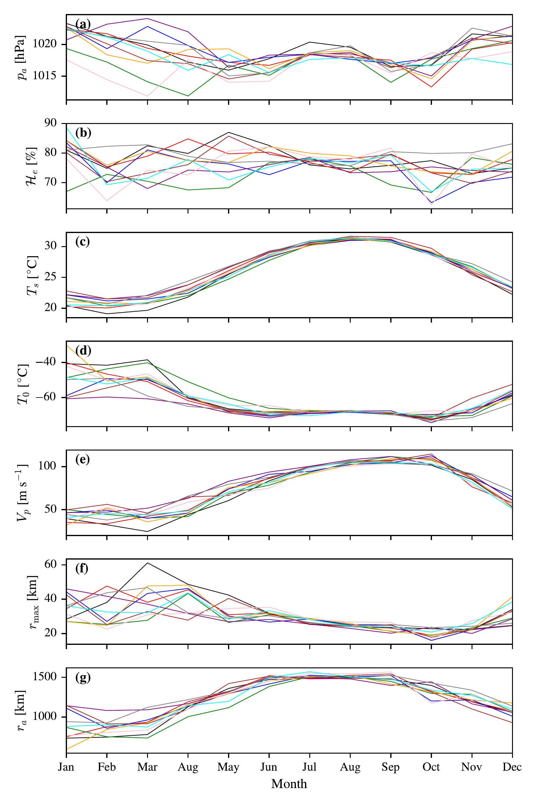
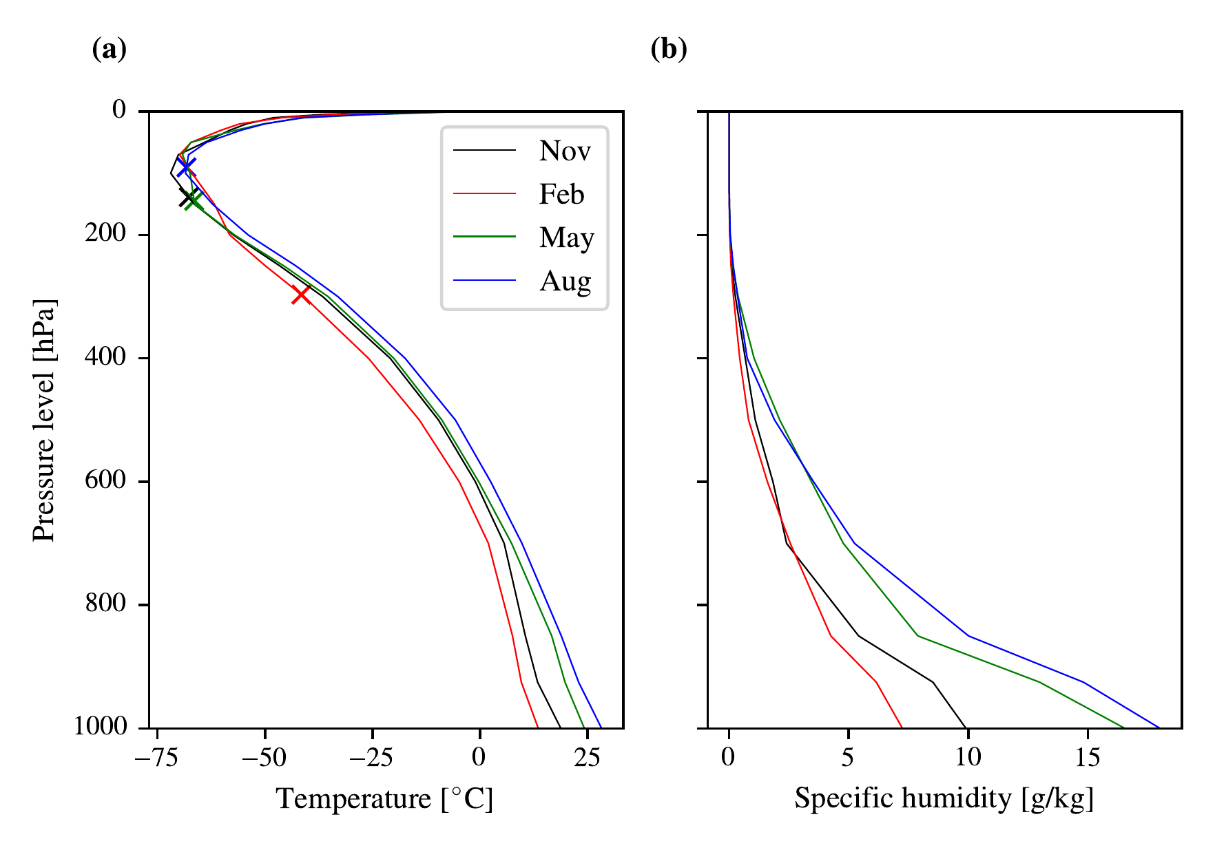
We use the inputs from the August monthly average because this around the peak of the hurricane season activity, and also around the peak for potential intensity, \(V_{p}\). To illustrate this see Figure 3.13 where we show the variation of potential intensity and its inputs over ten years of a CMIP6 ensemble member for the point closest to New Orleans (\(-90.25^{\circ}\text{E},\; 29.25^{\circ}\text{N}\)). As shown, for this point the potential intensity, \(V_p\), tends to peak in September, whereas the potential size, \(r_a\), has flat peak from roughly June to September. Figure 3.14 shows the corresponding vertical profiles for some of the months from the first year of the ensemble member. As shown, the outflow level rises to roughly the temperature inversion pressure level in August 2015, from a much lower level in February 2015.
The calculation of potential size is quite slow, taking around two
minutes per grid point per time point. This is partially because the
CLE15 profile calculation code is written in matlab (Chavas 2022), and
was ran by octave at each new guess of \(\tilde{r}_a\), which involves a launching
cost. To pass the input data to and from octave, a json
file is saved and its name is passed. Each point can be parallelized
onto a separate CPU, but this still makes the calculations too slow to
easily run for large CMIP6 datasets. It should be possible to improve
this in future by writing this purely in optimized python or another
language.
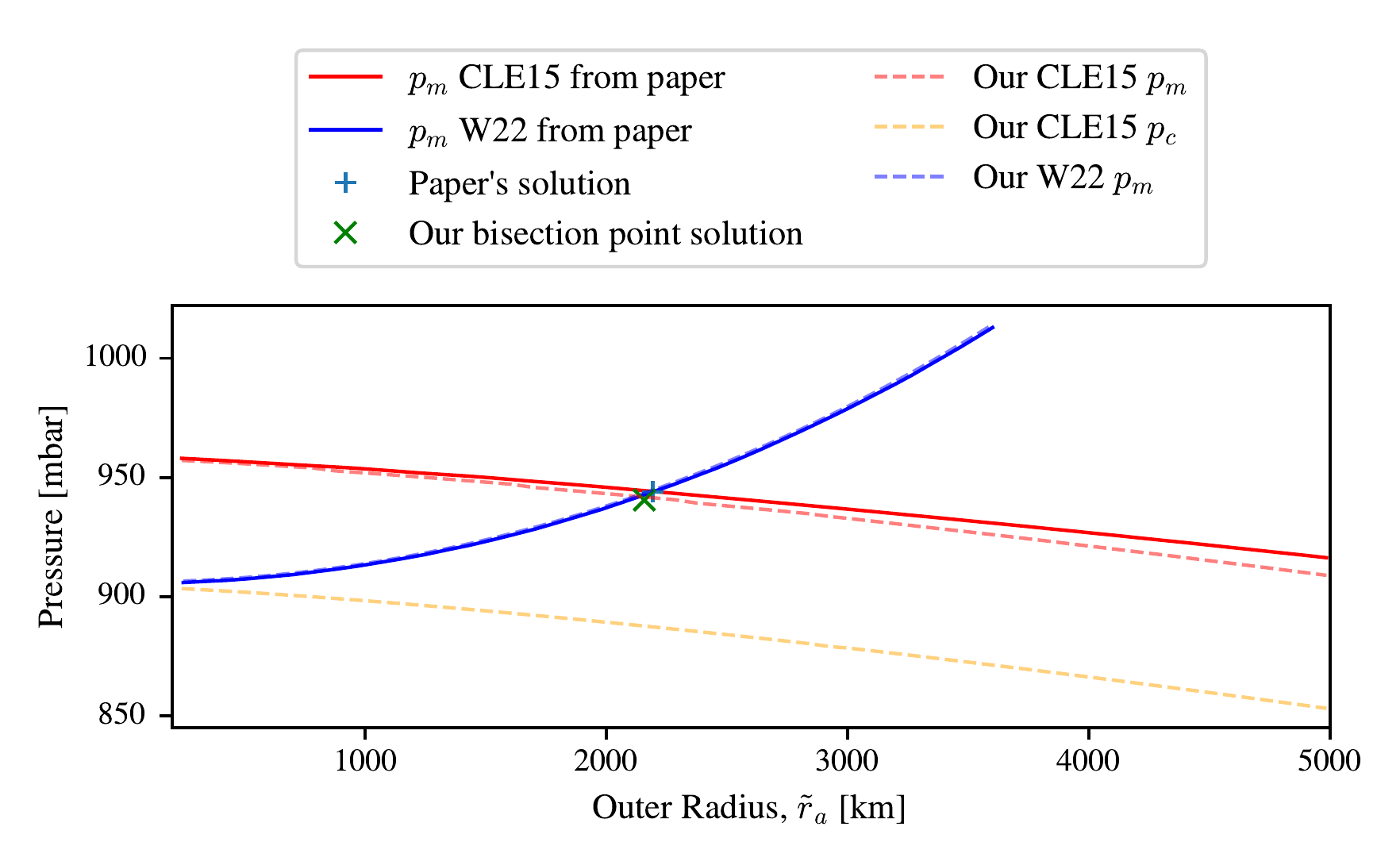
scipy.integrate. The pressure from the CLE15 profile at the
maximum winds is slightly lower in our solution than theirs, which may
be caused by our choice of integration method, or that they used a
higher (unreported) density. \(p_c\) is
the central pressure of the TC in the CLE15 model which is roughly a
constant 50 mbar lower than the pressure at the radius of maximum winds,
\(p_m\).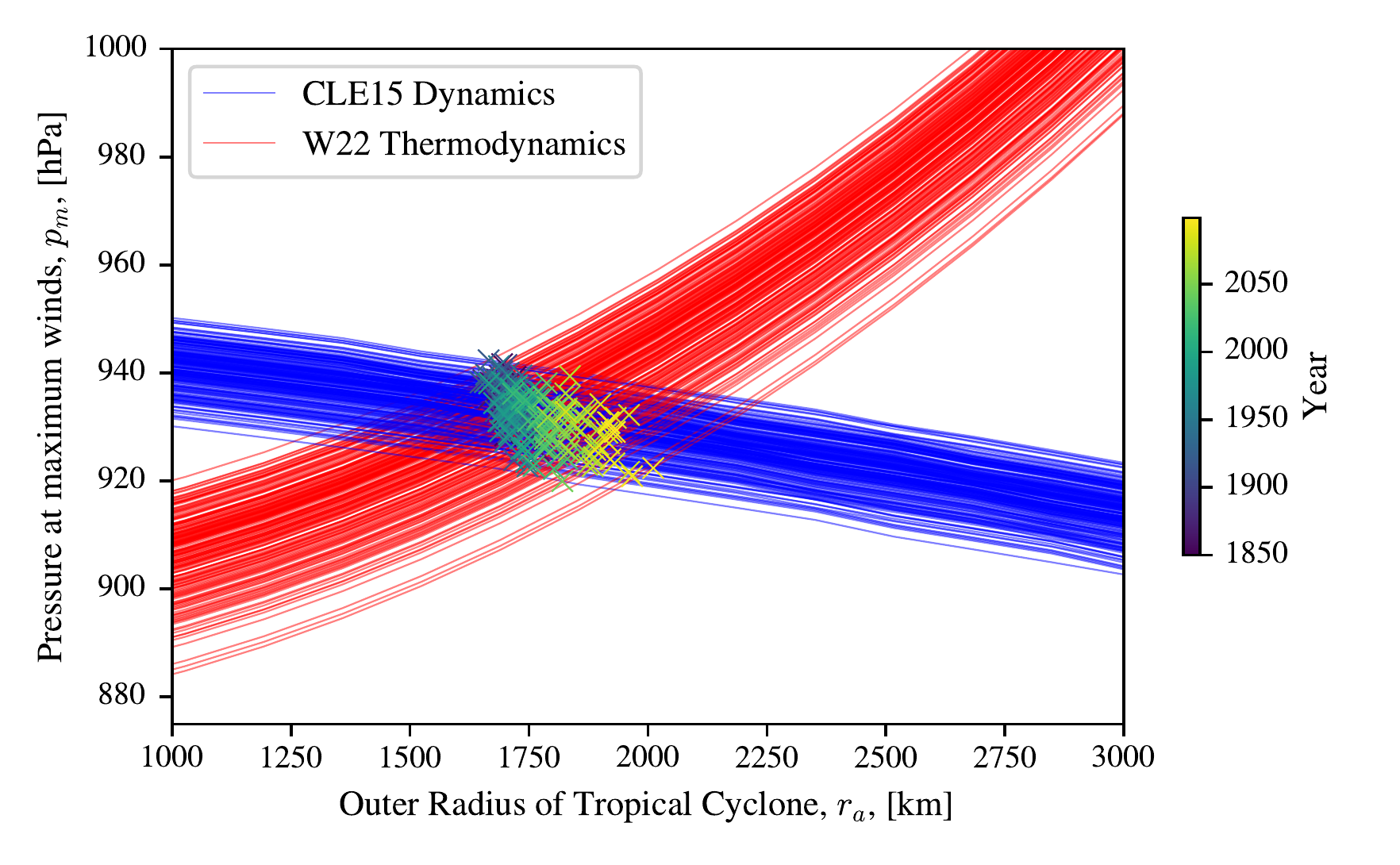
3.7 Appendix: ADCIRC model setup
We apply the atmospheric forcing in ADCIRC with netCDF4 files using the NWS=13 input setting. The inputs are the 10m zonal wind (U10) in m s\(^{-1}\), the 10m meridional wind (V10) in m s\(^{-1}\), and the surface pressure (PSFC) in mbar. The 10m windspeed \(\left|\vec{U}_{10}\right|\) is calculated as a constant factor \(V_{\mathrm{reduc}} =0.8\) of the gradient wind, \(V\left(r \right)\), and the surface pressure is calculated as in Equation Equation (3.10) using the gradient rather than the 10m wind. If each point in the mesh is at position \(\vec{p}\) and the centre of the TC is at position \(\vec{p}_c\), we calculate the distance from the centre for each point, \(r =\left|\left|\vec{p}-\vec{p}_c\right|\right|\), and its angle \(\phi=\arctan2\left(p_{x}-p_{cx},\; p_{y}-p_{cy}\right) - \pi / 2\), so that the 10m wind vector becomes, \[\begin{equation} \left(U10\left(\vec{p}\right),\; V10\left(\vec{p}\right)\right) = \left(\sin\left(\phi\right) \cdot V\left(r\right) \cdot V_{\mathrm{reduc}},\; \cos\left(\phi\right) \cdot V\left(r\right) \cdot V_{\mathrm{reduc}} \right), \end{equation}\](3.12) and defaults to \((0, 0)\) if \(r > r_a\). Similarly the pressure field is \(\mathrm{PSFC}=p(d)\), and defaults to \(p_a\) when \(r > r_a\).
The straight-line constant bearing trajectory of the TC is calculated so that it makes hits the impact location \(\vec{p}_i\) at the impact time \(t_i\). The impact location \(\vec{p}_i\) is defines as the observation location \(\vec{p}_o\) minus the track displacement, \(c\), so that \(\vec{p}_i=\left(p_{ox}-c, p_{oy}\right)\). The TC trajectory passes at translation speed \(V_t\) at track bearing \(\chi\) from due north, so that the position of the centre of the track, \(\vec{p}_c\), at time \(t\) is \(\vec{p}_c=\vec{p}_i + \left(t-t_i\right)\cdot V_t\cdot \left(\sin\left(\chi\right),\; \cos\left(\chi\right)\right)\).
These are input on two rectangular lat-lon grids: a coarser static grid (\(\frac{1}{8}^{\circ}\)), and a higher resolution moving grid centred on the TC centre \(\frac{1}{80}^{\circ}\). The purpose of the higher resolution moving grid is to better resolve the centre of the TC and decrease the errors brought about by interpolation in each time slice, as the interpolation algorithm used between input timesteps is movement aware. Using the NWS=13 setup also makes the ADCIRC run more flexible so that any cyclone, including arbitrarily asymmetric cyclones could be applied, alongside a background climatology, so that we can easily extend this framework to more realistic conditions.
S. Wang et al. (2022) found that forcing the ADCIRC model with the axisymmetric CLE15 profile, with a background wind model for the asymmetric component (Lin and Chavas (2012), referred to as LC12), significantly outperformed more standard parametric profiles such as the revised Holland profile (Holland et al. 2010) in the same setup, particularly for the more extreme storm surges. Chaigneau et al. (2024) showed that forcing ADCIRC with the CLE15 profile outperformed forcing it with ERA5 data, and was comparable to parametric models such as the generalized asymmetric Holland model (GAHM).
Each of our runs involves seven virtual days of simulation time. The tides have been turned off, and there is one day of linear ramping at the start of the meteorological data to avoid a hard shock of the new imposed conditions from creating transient effects. The run is parallelized across an Archer2 node with 128 CPUs and each ADCIRC run takes around three minutes.
For the Bayesian optimization experiments in the New Orleans region we apply the constraints that the TC broadly comes from the south, \(\chi\in \left(-80^{\circ},\; 80^{\circ}\right)\), the TC hits the region of the observation point, \(c\in\left(-2^{\circ}\text{E},\; 2^{\circ}\text{E}\right)\), and the translation speed is positive, and up to twice the translation speed of Hurricane Katrina at Landfall, \(V_t\in\left(0\text{ m s}^{-1},\;15\text{ m s}^{-1}\right)\). Each of these decisions is somewhat arbitrary, particularly for the upper bound translation speed, \(V_t\), which can become much faster. Translation speed could also interact in a complex way with both the size and intensity of a TC. If \(15\text{ m s}^{-1}\) is too low an upper bound, this would likely lead to an underestimate in the potential height for the open coastlines, but these are not the areas of the coast that were at the risk of the highest surges in Section Section 3.3.
3.8 Appendix: Investigating GEV fit sensitivity to the scale and shape parameters
In Figure 3.17, we compare the sizes of the bias and 5%–95% resampling ranges from the max known fit (I) and the max unknown fit (II) for the same return levels highlighted in Figure 3.10. We vary the values of the shape parameter, \(\gamma\), and the scale parameter, \(\beta\) chosen for the true GEV systematically for a plausible number of observations, \(N_s=50\). We keep the resamples constant \(N_r=600\), and vary \(\gamma\) between -0.1 and -0.4, and \(\beta\) between 0.2 m and 1.5 m. The biases in the estimate of the return value is much smaller for (I) than (II) (Figure 3.17(a),(f),(c),(h)), and the 5%–95% resampling ranges are also smaller (Figure 3.17(b),(g),(d),(i)). This is shown systematically in Figure 3.17(e)&(j) where the natural logarithm of the 5%–95% range for (II) divided by (I) is almost always positive. This illustrates that for a plausible size of the observational dataset, assuming block maxima, the 1 in 500 year return value in particular can be estimated much more accurately if the upper bound were known ahead of time, independent of the values of the shape and scale parameters, \(\gamma\) and \(\beta\).