Chapter 2
The potential intensity and potential sizes of tropical cyclones under climate change
Abstract. While tropical cyclone (TC) potential intensity has often been compared against observations and projected into the future, the same is not true of the recently proposed TC potential size. To improve this, we calculate TC potential intensity and potential sizes using monthly ERA5 data corresponding to the TC tracks from the IBTrACS observational dataset in the satellite era (1980–2024). We show that under some conditions, the potential size measure does seem to be predictive of the maximum size of TC radius of maximum winds. However, we also show that storms can become superintense and supersized, where the assumptions made in the potential intensity and potential size models no longer hold, such as after a suspected extratropical transition. We then calculate the trends in potential sizes and potential intensity over the satellite era in ERA5. As expected, we find that TC potential intensity generally increases due to global warming, as does the TC potential size of the weakest storms (at category 1 intensity), but we find that the TC potential size of the most intense storms at their TC potential intensity does not significantly change in most places in ERA5. We then find that the CMIP6 models we use have similar potential intensity and potential sizes over the satellite era to ERA5, and therefore use the SSP5-8.5 CMIP6 scenario to estimate how the potential size and potential intensity of TCs could change in the future. We examine two significant locations near New Orleans and Hong Kong and find that they project substantial increases in potential intensity and all potential sizes. This is an important contribution as there is no consensus on the future changes in TC size under climate change. This Chapter builds the thermodynamic variables that we can use to constrain TC storm surges in Chapters 3 and 4.
Impact Statement. Tropical cyclones are a major hazard to life and property, and it is important that we study how their size and intensity will change in the future. We compare a proposed limit to the size of a tropical cyclone against observations. This model predicts that, under the same conditions, if a storm is less intense it can grow larger. We show that the potential size of a cyclone at its observed windspeed provides a reasonable estimate of the maximum size of tropical cyclones. This suggests that this potential size measure could be used to help assess how the future risk of tropical cyclones will change as a result of climate change for various resultant perils, such as storm surges.
2.1 Introduction
Tropical cyclones (TCs) are powerful, rotating storm systems that form over tropical1 or subtropical2 waters. TCs are distinguished by the approximate azimuthal symmetry of their structure and a central, often cloud-free, eye surrounded by a towering eyewall. Known regionally as hurricanes in the North Atlantic and Northeast Pacific, and typhoons in the Northwest Pacific, these storms are massive heat engines that convert thermal energy from the ocean into destructive kinetic energy (Emanuel 1991). Their genesis requires a specific set of environmental conditions: high sea surface temperatures (at least 26.5\(^{\circ}\)C to a depth of 50m (Dare and McBride 2011)), atmospheric instability, high mid-tropospheric humidity, and sufficient distance from the equator (\(>5^{\circ}\)N or S) for the Coriolis force to be significant (Gray 1968).
TCs do not form spontaneously; they require a finite-amplitude seeding event, such as an African easterly wave, to nucleate. Once initiated, the dominant and most widely accepted paradigm for TC intensification is wind-induced surface heat exchange (WISHE): stronger surface winds drive greater latent and sensible heat flux from the ocean, increasing the thermodynamic disequilibrium that fuels the storm and further amplifying the winds in a positive feedback (Emanuel 1986, 1989; Rotunno and Emanuel 1987). The potential intensity and potential size theories we develop in this Chapter are grounded in WISHE thermodynamics. Earlier paradigms, conditional instability of the second kind (CISK, Charney and Eliassen 1964) and cooperative intensification (Ooyama 1969), can be understood as precursors that treat the ocean as a passive moisture source; WISHE superseded them by recognising the active, wind-speed-dependent role of air-sea enthalpy exchange. While there is some debate surrounding WISHE, with Montgomery et al. (2015) proposing a rotating convection paradigm in which intensification is instead driven by the organised aggregation of vortical hot towers (VHTs) within a “marsupial pouch” precursor disturbance (Dunkerton et al. 2009; Montgomery et al. 2006), the WISHE framework remains the basis of the thermodynamic potential intensity theory (Bister and Emanuel 2002) used throughout this Chapter.
Globally, around \(90 \pm 10\) TCs form each year (Maue 2011) and around half intensify to category 1 windspeed or above (33 m s\(^{-1}\), Maue 2011). Most GCM projections indicate a future reduction in global TC frequency, with increased wind shear (Vecchi and Soden 2007), reduced mid-level humidity (Tang and Emanuel 2012), and upper-tropospheric stabilisation (Santer et al. 2005) suppressing genesis despite higher SSTs; the signal persists in higher-resolution HighResMIP models (Roberts et al. 2020) and in fixed-SST CO\(_2\)-only experiments (Held and Zhao 2011). However, confidence remains limited: all evidence is GCM-derived, and observational detection is frustrated by the shortness of the satellite record (Knutson et al. 2019) and by aerosol forcing, which has driven substantial multi-decadal variability that obscures any greenhouse-gas-driven trend (Dunstone et al. 2013). The frequency reduction is therefore better treated as a plausible working hypothesis than an established result (Knutson et al. 2020). Nevertheless, other TC properties are robustly changing, with a greater proportion of storms reaching high intensities (Knutson et al. 2020; Seneviratne et al. 2021; Wehner and Kossin 2024).
As TCs are fueled by the thermodynamic disequilibrium between the warm sea surface and the cooler upper atmosphere (Emanuel 1986), a contrast enhanced by the greenhouse effect: warmer sea surfaces increase both the surface-to-outflow temperature gradient and, via the Clausius-Clapeyron relation, the enthalpy disequilibrium between ocean and atmosphere that fuels TC intensification (Emanuel 1987). It is therefore expected that TCs will have more available energy as greenhouse gas concentrations increase (we explore this further in Section Section 2.2.1.5). Projections indicate a future with more intense storms, higher rainfall rates, and a greater proportion of cyclones reaching the highest categories of intensity (Seneviratne et al. 2021). The intensity of a TC is often defined as the maximum sustained surface windspeed, which can be quantified as the azimuthal mean windspeed, \(V_{\mathrm{max}}\), at the radius of maximum winds, \(r_{\mathrm{max}}\). The Saffir-Simpson hurricane wind scale is commonly used to categorise TCs based on their maximum sustained wind speed, with categories ranging from 1 (weakest) to 5 (strongest).
To accommodate the increasing intensity of the strongest storms observed in a warming climate, an additional category 6 has been proposed for TCs with maximum sustained wind speeds above 86 m s\(^{-1}\) (309 km hr\(^{-1}\), 192 mile hr\(^{-1}\), Wehner and Kossin 2024). The lower boundaries of the revised Saffir-Simpson hurricane wind scale are shown in Table 2.1, which we use as a guide to describe TC windspeeds in the rest of this Chapter.
| Category | Lower Wind Speed Boundary | |||
| [m s\(^{-1}\)] | [km hr\(^{-1}\)] | [mile hr\(^{-1}\)] | [knots] | |
| 1 | 33 | 119 | 74 | 64 |
| 2 | 43 | 154 | 96 | 83 |
| 3 | 50 | 177 | 111 | 96 |
| 4 | 58 | 209 | 130 | 113 |
| 5 | 70 | 252 | 157 | 137 |
| 6 | 86 | 309 | 192 | 167 |
Emanuel (1986) introduces the concept of TC potential intensity, which is the maximum intensity a TC can achieve given the environmental conditions, a theory further refined in Emanuel (1995; Bister and Emanuel 1998; Bister and Emanuel 2002). Emanuel (2000) analyse the distribution of TC intensities as a fraction of their potential intensity, \(V_p\), finding that the maximum wind speed of observed storms is indeed capped at approximately the potential intensity along their track.
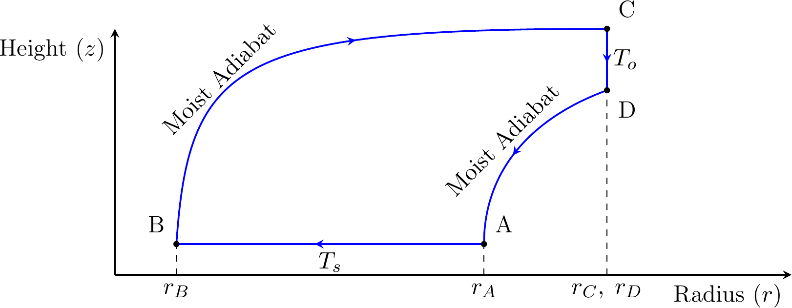
However, the destructive potential of a TC is a function of its entire radial structure, not just its peak winds. We therefore introduce the key radial scales used throughout this Chapter. The outer radius, \(r_A\), is defined as the radius at which the azimuthal wind speed vanishes, in other work it is sometimes measured by the last closed isobar of the cyclone. In the theoretical Chavas et al. (2015) model this is an exact zero-wind boundary; observationally the wind decays asymptotically, so a small threshold (e.g. 2 m s\(^{-1}\)) is used in practice. The radius of maximum winds, \(r_{\max}\) (labelled \(r_B\) in the Carnot engine cycle of Figure 2.1), is the radius at which the azimuthal wind reaches its peak value \(V_{\max}\). Throughout this Chapter, \(V_{\max}\) denotes the 10 m sustained wind speed; gradient-level quantities carry distinct symbols: \(V_p\) for potential intensity and \(V_{gm}\) for the Chavas et al. (2015) wind profile.
The pressure deficit \(\Delta p\) used in this Chapter is the sea-level pressure difference between the outer boundary and the radius of maximum winds, \[\begin{equation} \Delta p = p(r_A) - p(r_{\max}). \end{equation}\](2.1) This differs from the more common central pressure deficit \(\Delta p_c = p(r_A) - p(0)\), which extends the integral all the way to the eye. We adopt the \(r_{\max}\)-referenced definition because the potential size model of D. Wang et al. (2022) is formulated in terms of the pressure at the radius of maximum winds, making Equation (2.1) the natural choice for consistency. Under gradient wind balance, \(\Delta p\) integrates the azimuthal wind field from \(r_A\) to \(r_{\max}\) (Chavas et al. 2017), and therefore captures both the intensity and the outer size of the storm in a single scalar, so is a more holistic metric than \(V_{\max}\) alone. The Saffir-Simpson scale’s focus on \(V_{\max}\) can thus be misleading, as it neglects other hazards like storm surge and rainfall that are strongly influenced by overall storm size (Zhai and Jiang 2014).
D. Wang et al. (2022, 2023) introduce the concept of TC potential size, which they describe as the maximum size a TC’s outer radius can achieve given the environmental conditions (which we call the potential outer size), based on combining energetic and dynamic constraints. We first attempt similar analysis to Emanuel (2000) using adapted forms of D. Wang et al. (2022) for the radius of maximum winds (which we call the potential inner size) so that they are easier to compare against historical best track observations. We then seek to show whether our measures of potential size also show significant trends over historical observations and climate change projections, and therefore seek to answer whether we should expect the maximum size of TCs to increase with global warming, and how similar this effect is compared to potential intensity.
This Chapter advances from D. Wang et al. (2022) by:
Reformulating their model as a way to calculate the radius of maximum winds, i.e. the potential inner size, under different assumptions of intensity, as an intensity–size tradeoff for each ocean grid point in a climate model output. We additionally define special radii: the category 1 intensity potential inner size (Cat1 PS, \(r_1\)), the corresponding (observed) intensity potential inner size (CPS, \(r_2\)), and the potential intensity potential inner size (PI PS, \(r_3\)).
Validating this \(r_{\max}\) prediction against the IBTrACS observations by assuming the observed intensity, and then verifying that there appears to be a domain of validity (roughly \(10^{\circ}\)–\(30^{\circ}\) latitude) where the model usefully bounds the inner size.
Using the model to calculate the trends and spatial patterns of potential sizes for both ERA5 and CMIP6 in the historical period (noting biases), and for SSP5-8.5 for CMIP6.
These tasks provide the thermodynamic data we need to calculate the worst possible storm surge (the potential height) in later Chapters 3 and 4.
In Section Section 2.2 we first outline the derivations for the key variables of potential intensity (Section Section 2.2.1) and potential size (Section Section 2.2.2). We then outline the methodology used to calculate the potential intensity and potential size of TCs in Section Section 2.3.1. Finally, we present the results of our analysis in Section Section 2.4 and discuss the implications of our findings in Section Section 2.6. One of the key contributions of the Chapter is the new Python implementation of the Chavas et al. (2015) radial wind profile model, and of the potential size model more broadly, available in Thomas (2025), and discussed in Appendix Section 2.8.
2.2 Background Theory
2.2.1 Potential intensity
2.2.1.1 Summary
The potential intensity, \(V_p\), of a TC is the proposed maximum azimuthal gradient wind speed that a TC can achieve given the environmental conditions at its radius of maximum wind speed, \(r_{\mathrm{max}}\). This is calculated following Bister and Emanuel (2002) as \[\begin{equation} \left(V_{p}\right)^2 = \frac{T_s}{T_o}\frac{C_h}{C_d} \left(\text{CAPE}_B^{*} - \text{CAPE}_{A}\right), \end{equation}\](2.2) where \(V_{p}\) is the potential intensity at the gradient wind level, i.e. no reduction to 10 m winds is applied, \(\text{CAPE}_B^{*}\) is the convective available potential energy of saturated air lifted from the sea surface to the outflow level, \(\text{CAPE}_{A}\) is the convective available potential energy of the environment, \(C_h\) is the enthalpy exchange parameter, \(C_d\) is the momentum exchange parameter, \(T_s\) is the surface temperature, and \(T_o\) is the outflow temperature. This is derived by assuming a simple Carnot engine between the sea surface and the level of neutral buoyancy (roughly the tropopause), we provide a brief derivation here.
= [thick, blue, postaction=decorate, decoration=markings, mark=at position 0.55 with ] = [thick,->,>=stealth]
2.2.1.2 Derivation of potential intensity
2.2.1.2.1 Problem Set Up
To simplify the treatment, we do not follow the original derivation from Emanuel (1986, 1995; Bister and Emanuel 1998; Bister and Emanuel 2002). Instead, we use the simpler derivation in Makarieva et al. (2018). We assume that the TC is in its limit a Carnot engine shown in Figure 2.1 where the heat is absorbed as the air parcel isothermally flows into the center of the storm. The parcel then rises adiabatically at the eyewall up to the outflow level (B-C), where the air cools adiabatically during descent at \(T_o\) (C-D), and then finally descends adiabatically back to the sea surface at point \(A\), (D-A). The heat input from the ocean during the first process (A-B) drives the system, while the heat loss to space during the third process (C-D) represents the cooling of the outflow air. The cycle represents the energy transfer and thermodynamic processes in a TC.
2.2.1.2.2 Defining Thermodynamic Variables
The first law of thermodynamics can be written as \(Tds=dh-\alpha dp\), where \(T\) [K] is the temperature, \(s\) [J kg\(^{-1}\) K\(^{-1}\)] is the specific entropy, \(h\) [J kg\(^{-1}\)] is the specific moist enthalpy (the internal energy of the parcel), \(\alpha\) [m\(^3\) kg\(^{-1}\)] is the specific volume, and \(p\) [Pa] is the pressure. The specific moist enthalpy, \(h\) [J kg\(^{-1}\)], is defined as, \[\begin{equation} h = c_p T + L_v q, \end{equation}\](2.3) where \(c_p\) [J kg\(^{-1}\) K\(^{-1}\)] is the specific heat capacity at constant pressure, \(L_v\) [J kg\(^{-1}\)] is the latent heat of vaporisation, and \(q\) [kg kg\(^{-1}\)] is the specific humidity. In other words the internal energy of the parcel comes from the ideal gas being at its temperature, \(T\), and the latent heat of the water vapour in the parcel at its specific humidity, \(q\). Therefore the first law of thermodynamics becomes, \[\begin{equation} T ds = c_p dT + L_v dq - \alpha dp. \end{equation}\](2.4) We can further assume that the air will approximately follow the ideal gas law for a dry parcel \(p_d\alpha=R_d T\), where \(p_d\) [Pa] is the partial pressure of dry air and \(R_d\) [J kg\(^{-1}\) K\(^{-1}\)] is the specific gas constant for dry air. Since specific humidity in the tropics is typically \(q \lesssim 0.02\) kg kg\(^{-1}\) \(\ll 1\), the dry air dominates the thermodynamic behaviour and \(p_d \approx p\), so \(\alpha dp\approx \left(R_d T / p_d \right) dp\). This becomes \[\begin{equation} T ds \approx c_p dT + L_v dq - \frac{R_d T}{p_d} dp. \end{equation}\](2.5) and then assuming that the dry pressure is approximately equal to the total pressure \(p_d \approx p\), \[\begin{equation} ds \approx c_p \frac{dT}{T} + L_v\frac{1}{T}dq - R_d \frac{1}{p}dp, \end{equation}\](2.6) which, when integrated and ignoring constants, gives the entropy of the parcel \[\begin{equation} s \approx \underbrace{c_p \ln T}_{\text{Dry air temperature contribution}} + \underbrace{\frac{L_v q}{T}}_{\text{Latent heat contribution}} - \underbrace{R_d \ln p}_{\text{Pressure contribution}}. \end{equation}\](2.7)
2.2.1.2.3 Finding the Net Work Done
If we assume the TC is a perfect Carnot engine, then the net work done, \(W_{\mathrm{net}}\), must equal the net heat input over the cycle \(\oint T ds\) as the cycle is closed and energy is conserved, \[\begin{equation} W_{\mathrm{net}} = \oint Tds. \end{equation}\](2.8) We can then break it into the four legs of the cycle, so we have \[\begin{equation} W_{\mathrm{net}} = \oint Tds = \int_{A}^{B} T ds + \int_{B}^{C} T ds + \int_{C}^{D} T ds + \int_{D}^{A} T ds. \end{equation}\](2.9) The adiabatic legs B-C and D-A contribute nothing to the integral, since moist adiabatic ascent and descent conserve entropy (\(ds=0\) along an isentrope, so \(\int T\,ds=0\) on both legs), leaving just the isothermal legs A-B and C-D. Additionally this means we know that \(s_B=s_C\) and \(s_D=s_A\), so that we have, \[\begin{align} W_{\mathrm{net}} &= \int_{A}^{B} T ds + \int_{C}^{D} T ds\\ &= \int_{A}^{B} T_s ds + \int_{C}^{D} T_o ds \\ &=Q_{\mathrm{in}} + Q_{\mathrm{out}}\\ &= (s_B- s_A) T_s + (s_D- s_C) T_o \\ &= \left(s_C - s_A\right) T_s + \left(s_A - s_C\right) T_o \\&= \left(s_C - s_A\right) \left(T_s - T_o\right). \end{align}\](2.10) The heat input to the Carnot engine is given by the entropy change along the inflow isotherm \[\begin{equation} Q_{\mathrm{in}} = \int_{A}^{B} T_s ds = \left(s_C - s_A\right) T_s, \end{equation}\](2.11) which means that \[\begin{equation} W_{\mathrm{net}} = Q_{\mathrm{in}} \frac{T_s - T_o}{T_s} = Q_{\mathrm{in}} \epsilon_{s}, \end{equation}\](2.12) where \(\epsilon_{s}\) is the efficiency of the Carnot engine \[\begin{equation} \epsilon_{s} = \frac{T_s - T_o}{T_s}. \end{equation}\](2.13)
2.2.1.2.4 The Carnot Engine’s Inflow
We assume all heat enters the engine at the inflow A-B. Since leg A-B is isothermal at \(T_s\), the entropy change \(ds = dh/T_s - \alpha\,dp/T_s\) receives contributions from both the increase in specific humidity \(q\) (latent heat uptake) and the inward pressure decrease (\(p_B < p_A\), giving a term \(-R_d\ln(p_B/p_A)>0\)); the latter is retained explicitly below and later dropped as a small correction. The enthalpy changes from \(h_A\) at point A to \(h_B^{*}\) (where \({}^*\) denotes saturation) at point B. The enthalpy change along the isothermal leg A-B is given by, \[\begin{equation} h_B^{*} - h_A = L_v \left(q_B - q_A\right), \end{equation}\](2.14) and the entropy change over this leg is \[\begin{equation} s_B^{*} - s_A = \frac{L_v \left(q_B - q_A\right)}{T_s} - R_d \ln \frac{p_B}{p_A} = \frac{Q_{\mathrm{in}}}{T_s}. \end{equation}\](2.15) If we ignore the entropy change due to pressure in this leg as small then we can make the approximation, \[\begin{equation} Q_{\mathrm{in}} = T_s\left(s_B^{*} - s_A\right) \approx L_v \left(q_B - q_A\right) = h_B^{*} - h_A. \end{equation}\](2.16) For very intense TCs, the pressure term \(-R_d T_s \ln(p_B/p_A)\) can reach 10–20% of the latent-heat contribution; however, the CAPE-based formulation in the next section avoids this approximation by computing the heat input directly from environmental soundings.
2.2.1.2.5 Finding Potential Intensity through Assessing the Carnot Engine in Steady State
Now that we have found the Carnot engine’s efficiency and heat input, we can further assume that the cycle is at steady state. The efficiency of the Carnot engine must also apply to the rate of work done against the sea surface, \(D\) [W m\(^{-2}\)], and the rate of heat input, \(H\) [W m\(^{-2}\)], so that \[\begin{equation} {D}=\epsilon_{s} H. \end{equation}\](2.17) We can either assume that the heat input \(H\) comes purely from sea air enthalpy exchange \(J_h\) [W m\(^{-2}\)] (assumption I, as originally assumed in Emanuel (1986)) or we can assume that the work against the sea surface, \(D\), is also transformed into heat so that \(H=J_h+D\) (assumption II introduced in e.g. Bister and Emanuel (1998; Bister and Emanuel 2002)), and therefore \(D=\epsilon_{s} \left(J_h+D\right)\). We use assumption II, so that \[\begin{equation} D = \frac{\epsilon_{s}}{1-\epsilon_{s}}J_h, \end{equation}\](2.18) where \(D\) [W m\(^{-2}\)] is the kinetic energy dissipation rate per unit area by boundary-layer surface friction, and \(J_h\) [W m\(^{-2}\)] is the turbulent air-sea enthalpy flux, the bulk aerodynamic exchange of sensible and latent heat between the ocean surface and the overlying atmosphere. Given that \(\epsilon_{s}=\frac{T_s-T_o}{T_s}\), the new efficiency prefactor becomes \(\epsilon_{0} = \frac{\epsilon_{s}}{1-\epsilon_{s}}=\frac{T_s-T_o}{T_o}\), so recycling the frictional dissipation back into the cycle (assumption II) simply replaces \(T_s\) with \(T_o\) in the denominator. We assume that both \(D\) and \(J_h\) are overwhelmingly dominated by the processes occurring near the radius of maximum winds, so that we consider a single velocity, \(V\), at the radius of maximum winds, \(r\).
The kinetic energy dissipation rate, \(D\), is given by \[\begin{equation} D = \rho C_d V^3, \end{equation}\](2.19) where \(\rho\) [kg m\(^{-3}\)] is the air density and \(C_d\) [\(-\)] is the dimensionless drag coefficient. The rate of enthalpy exchange is given by the bulk aerodynamic formula \[\begin{equation} J_h = \rho C_h V\left(h_B^{*}-h_A\right), \end{equation}\](2.20) where \(h_B^{*}\) [J kg\(^{-1}\)] is the saturated enthalpy at the sea surface, \(h_A\) [J kg\(^{-1}\)] is the enthalpy of the ambient air, and \(C_h\) [\(-\)] is the dimensionless enthalpy exchange coefficient (analogous to a Stanton number), a transfer efficiency, not a heat transfer coefficient in W m\(^{-2}\) K\(^{-1}\). This could be seen as an aggressive assumption, as it is equivalent to assuming that the air parcel is dropped directly at the radius of maximum winds to exchange enthalpy, which will increase the resultant potential size. Therefore we have \[\begin{equation} \rho C_d V ^3 = \frac{T_s-T_o}{T_o} \rho C_h V\left(h_B^{*}-h_A\right). \end{equation}\](2.21) Dividing both sides by \(\rho C_h V\) we have the expression for potential intensity from Bister and Emanuel (1998), \[\begin{equation} V ^2 = \frac{T_s-T_o}{T_o} \frac{C_h}{C_d}\left(h_B^{*}-h_A\right). \end{equation}\](2.22)
2.2.1.2.6 Introducing the Convective Available Potential Energy (CAPE)
The convective available potential energy, CAPE, is defined as the integral of the parcel’s positive buoyancy from the sea surface to the level of neutral buoyancy (LNB), which is roughly the tropopause for most TCs. CAPE is given by \[\begin{equation} \text{CAPE} = \int_{z_s}^{z_{\mathrm{LNB}}} g\left(\frac{\theta_v-\theta_{v,\mathrm{env}}}{\theta_{v,\mathrm{env}}}\right) dz, \end{equation}\](2.23) where \(g\) is the acceleration due to gravity, \(\theta_v\) is the virtual potential temperature of the parcel, and \(\theta_{v,\mathrm{env}}\) is the virtual potential temperature of the environment. The CAPE can be approximated as \[\begin{equation} \text{CAPE} \approx \int^{p_{LFC}}_{p_{EL}}(\alpha_{\text{parcel}} - \alpha_{\text{env}}) dp, \end{equation}\](2.24) where \(p_{LFC}\) is the pressure at the level of free convection, \(p_{EL}\) is the pressure at the equilibrium level, \(\alpha_{\text{parcel}}\) is the specific volume of the parcel, and \(\alpha_{\text{env}}\) is the specific volume of the environment.
2.2.1.2.7 Relating CAPE to Net Work Done
We introduce CAPE by returning to the full net work done by the Carnot engine \[\begin{align} W_{\mathrm{net}} &= \oint Tds = \int_{A}^{B} T ds + \int_{B}^{C} T ds + \int_{C}^{D} T ds + \int_{D}^{A} T ds,\\ &= \int_{A}^{B} \alpha dp + \int_{B}^{C} \alpha dp + \int_{C}^{D} \alpha dp + \int_{D}^{A} \alpha dp. \end{align}\](2.25) Given that \(\alpha_e\) is the environmental specific volume we assume \(\oint \alpha_e dp = 0\). Therefore we can write \[\begin{equation} W_{\mathrm{net}} = \int_{A}^{B} \left(\alpha - \alpha_e \right) dp + \int_{B}^{C} \left(\alpha - \alpha_e \right) dp + \int_{C}^{D} \left(\alpha - \alpha_e \right)dp + \int_{D}^{A} \left(\alpha - \alpha_e \right)dp. \end{equation}\](2.26) The pressure change for the two isothermal legs (A-B, C-D) compared to the moist adiabatic legs (B-C, D-A), therefore \[\begin{equation} W_{\mathrm{net}} = \int_{B}^{C} \left(\alpha - \alpha_e \right) dp + \int_{D}^{A} \left(\alpha - \alpha_e \right) dp = \text{CAPE}_B^{*} - \text{CAPE}_A, \end{equation}\](2.27) where \(\text{CAPE}_B^{*}\) is the convective available potential energy of saturated air lifted from the sea surface at the radius of maximum winds to the outflow level, and \(\text{CAPE}_A\) is the convective available potential energy of unsaturated ambient air. We assume that the convective available potential energy consumed around the loop is equal to the enthalpy input, neglecting irreversible entropy production, such that \[\begin{equation} \text{CAPE}_B^{*} - \text{CAPE}_A \approx \frac{T_s-T_o}{T_s}\left(h_B^{*}-h_A\right) = \frac{\epsilon_{s} J_h}{\rho C_h V }, \end{equation}\](2.28) substituting into the into Bister and Emanuel (1998)’s expression for potential intensity (Equation (2.22)) gives \[\begin{equation} \left(V_{p}\right)^2 = \frac{T_s}{T_o}\frac{C_h}{C_d} \left(\text{CAPE}_B^{*} - \text{CAPE}_{A}\right). \end{equation}\](2.29) This is the potential intensity as defined in Bister and Emanuel (2002). Equally we could have reached the same result directly by substituting the bulk aerodynamic expressions \(D = \rho C_d V^3\) and \(J_h = \rho C_h V (h_B^* - h_A)\) into the dissipation balance \(D = \frac{\epsilon_s}{1-\epsilon_s} J_h\) and eliminating \(D\) and \(J_h\), bypassing the intermediate enthalpy route, by noting that \[\begin{align} D &= \frac{\epsilon_{s}}{1-\epsilon_{s}}J_h, \\ =C_d \rho V^3 & = \frac{1}{1-\epsilon_{s}}\left(\text{CAPE}_B^{*}-\text{CAPE}_A\right) \rho C_h V, \end{align}\](2.30) such that \[\begin{align} \left(V_{p}\right)^2 = \frac{T_s}{T_o}\frac{C_h}{C_d} \left(\text{CAPE}_B^{*} - \text{CAPE}_{A}\right). \end{align}\](2.31) If dissipative heating is ignored (assumption I, see e.g. Emanuel 1995) then we instead find \[\begin{equation} \left(V_{p}\right)^2 = \frac{C_h}{C_d} \left(\text{CAPE}_B^{*} - \text{CAPE}_{A}\right). \end{equation}\](2.32) The term \(\frac{T_s}{T_o}\) comes from \(\frac{\epsilon_{0}}{\epsilon_{s}}\), which comes from including the dissipative heating (assumption II). The term \(\frac{C_h}{C_d}\) comes from assuming that the rate of surface enthalpy flux times \(\epsilon_{0}\) is equal to the rate of kinetic energy dissipation at the radius of maximum wind.
2.2.1.3 Assumptions and limitations
Steady state (most limiting). The TC is assumed to have reached a steady thermodynamic equilibrium in which environmental conditions are constant. This is the most severe limitation: real TCs are highly transient, rarely sustaining steady-state conditions for more than a few hours (Emanuel 1995). As a consequence, observed TCs occasionally exceed their theoretical PI, a phenomenon known as superintensity, discussed further in Section Section 2.2.2.
Axisymmetry. The TC is assumed to be axisymmetric. In reality, vertical wind shear, land interaction, and outer rainbands introduce substantial asymmetries that suppress intensity below PI. The dominant mechanism is ventilation: wind shear tilts the vortex and imports low-entropy environmental air into the eyewall, diluting the warm core and reducing the Carnot engine’s effective heat input (Tang and Emanuel 2012). Storm translation adds a further asymmetry: faster-moving TCs develop a stronger forward quadrant and weaker rear quadrant, as surface winds are enhanced downwind of the vortex centre relative to the ground (Corbosiero and Molinari 2003).
Gradient wind and hydrostatic balance. The flow is assumed to be in gradient wind balance and in hydrostatic balance. Supergradient winds in the boundary layer violate the former, though the gradient-level PI remains a useful upper bound.
Constant exchange coefficients. The ratio of the enthalpy exchange coefficient, \(C_h\), and momentum exchange coefficient, \(C_d\), are treated as a constant (typically \(C_h/C_d \approx 0.9\) at high wind speeds). Observations suggest both vary with wind speed, sea state, and precipitation (Bister and Emanuel 2002).
Dry ideal gas approximation. The derivation uses \(p_d\alpha \approx R_d T\), the ideal gas law for dry air. Tropical specific humidities \(q \lesssim 0.02\) kg kg\(^{-1}\) mean this introduces errors of order \(q\ll 1\) in thermodynamic quantities, which are negligible under typical TC conditions.
2.2.1.4 Observational validation and applications
TC potential intensity (PI) is widely used to assess the intensity of TCs and to project future changes in TC intensity. Emanuel (2000) show that the maximum wind speed of TCs is capped at around the potential intensity along the track for those cyclones not limited by declining PI or landfall. Bister and Emanuel (2002) show that the PI is a good predictor of TC intensity, and that it can be used to assess the impact of climate change on TC intensity. Gilford (2021) introduced a Python package for calculating potential intensity using the Bister and Emanuel (2002) method, which has been widely used in the community.
A critical evolution in this understanding came from Vecchi and Soden (2007), who demonstrate that PI is not governed by local sea surface temperature (\(T_s\)) alone, but rather by the regional \(T_s\) warming relative to the tropical mean. This finding explained why observed trends in PI were not uniform despite widespread ocean warming. Subsequent research has leveraged more advanced reanalysis products and observational datasets to refine these trend estimates. A significant advancement has been the move from observing trends to attributing them to anthropogenic forcing. Bhatia et al. (2019) find that the observed increases in TC intensification rates in the Atlantic are statistically unusual and had a detectable contribution from anthropogenic factors, linking thermodynamic potential to observed storm behavior. This connection is further strengthened by work like Kossin et al. (2020), which identified a global increase in the proportion of major TCs (Category 3-5) over the past four decades, a trend consistent with a warming-induced increase in potential intensity.
2.2.1.5 Sensitivity analysis
To investigate the sensitivity of the expression for potential intensity to global warming, we can rewrite Equation (2.22) in a slightly simpler form with enthalpy difference \(\Delta h = h_B^{*} - h_A\), \[\begin{equation} V_p = \frac{T_s - T_o}{T_o} \frac{C_h}{C_d} \Delta h, \end{equation}\](2.33) so that we can easily conduct a sensitivity test. To quantify the response of TC potential intensity, \(V_p\), to a \(1^{\circ}\text{C}\) increase in global mean surface temperature (\(\Delta T_{\text{global}}\)): We assume (a) that tropical sea surface temperatures \(T_{s}\) heat some constant factor, \(n=0.8\), of the global average temperature change, \(\Delta T_{\text{global}}\), (b) that the outflow temperature warms up by some factor, \(m\), of the inflow temperature change3 and (c) that the enthalpy change scales with the Clausius-Clapeyron relationship for saturated specific humidity (\(k = 7\)% increase per degree kelvin) for that sea surface temperature. We can do this because the specific enthalpy of a parcel is defined as, \(h=L_v q + c_p T\), so \(\Delta h = h_B^{*} - h_A = L_v\left(q_B^{*} - q_B\right)= L_v \Delta q\) as the inflow is isothermal, and we assume \(\Delta q\) scales with \(q_B^{*}\), i.e. that the change in the saturation specific humidity is dominant. This is justified because \(\Delta q = q_B^{*}(1 - \mathcal{H})\), where \(\mathcal{H}\) is the ambient boundary-layer relative humidity; if \(\mathcal{H}\) remains approximately constant under warming, the standard Emanuel PI assumption supported by observations and models over the tropical ocean, then \(\Delta q\propto q_B^{*}\) and the Clausius–Clapeyron scaling applies directly. So in total, we have assumed the parameterization, \[\begin{align} T_{s} &= T_{s0} + n \Delta T_{\text{global}},\\ T_{o} &= T_{o0} + m \Delta T_{s},\\ \Delta h &= \Delta h_0 \left(1 + k \Delta T_{s}\right), \end{align}\](2.34) where \(\Delta h_0\) is the original enthalpy change, \(T_{s0}\) is the initial sea surface temperature, \(T_{o0}\) is the initial outflow temperature, and \(\Delta T_{s}\) is the change in sea surface temperature. Substituting the parameterization into \(V_p^2 \propto \frac{T_s - T_o}{T_o}\Delta h\) gives the warmed and baseline states as \[\begin{align} V_{p1}^2 &\propto \frac{(T_{s0}+\Delta T_s)-(T_{o0}+m\Delta T_s)}{T_{o0}+m\Delta T_s}\,\Delta h_0(1+k\Delta T_s) \\ &= \frac{T_{s0}-T_{o0}+(1-m)\Delta T_s}{T_{o0}+m\Delta T_s}\,\Delta h_0(1+k\Delta T_s),\\ V_{p0}^2 &\propto \frac{T_{s0}-T_{o0}}{T_{o0}}\,\Delta h_0. \end{align}\](2.35) Dividing and taking the square root yields the fractional change in wind speed \((V_{p1}/V_{p0})\). We then use the potential intensity expression from Equation (2.22) (Bister and Emanuel 1998), with the fractional change in wind speed (\(V_{p1}/V_{p0}\)) given by the equation, \[\begin{equation} \begin{split} \frac{V_{p1}}{V_{p0}} &= \frac{V_p\left(T_{\text{global}} = T_{g0} + \Delta T_{\text{global}}\right)}{V_p\left(T_{\text{global}} = T_{g0}\right)} \\ &= \sqrt{\frac{T_{s0} - T_{o0} + (1-m)\Delta T_{s}}{T_{o0} + m \Delta T_{s}} \cdot \frac{T_{o0}}{T_{s0} - T_{o0}} \cdot (1 + k \Delta T_{s})}, \end{split} \end{equation}\](2.36) where the initial state is defined by a sea surface temperature, \(T_{s0} = 300\,\text{K}\), and an outflow temperature, \(T_{o0} = 200\,\text{K}\).4 The sensitivity to upper-tropospheric (c. tropopause) warming was tested by varying the parameter \(m\), the ratio of outflow warming to surface warming as summarized in Table 2.2. For a \(1^\circ\text{C}\) global temperature increase (\(\Delta T_{s} = 0.8\,\text{K}\)), a value of \(m=1.0\) yielded a 2.56% increase in potential wind speed. Increasing the amplification factor to a more realistic \(m=1.2\) resulted in a 2.43% increase. For the most physically realistic scenario of strong moist adiabatic amplification, \(m=1.5\) (Santer et al. 2005), the model projects an increase in PI of 2.25%. If instead of assuming that the outflow temperatures increased, we assumed they decreased (e.g. \(m=-1\)) then the sensitivity would increase to 3.79% per degree of global warming, showing that if the tropopause cooled instead of warmed, this would dramatically increase our potential intensity sensitivity to warming. These results demonstrate that while increased enthalpy drives intensification, the final sensitivity is critically modulated by the degree of upper-tropospheric warming, with realistic assumptions yielding an estimate consistent with the 2–5% range projected by comprehensive climate models (Knutson et al. 2020).5
| \(n\) | \(m\) | \(k\) | Increase in \(V_p\) for \(1^\circ\text{C}\) global warming [%] |
|---|---|---|---|
| 0.8 | 1 | 0.07 | 2.56 |
| 0.8 | 1.2 | 0.07 | 2.43 |
| 0.8 | 1.5 | 0.07 | 2.25 |
| 0.8 | -1 | 0.07 | 3.79 |
2.2.2 Potential size
2.2.2.1 Summary and changes
D. Wang et al. (2022) introduce the concept of potential size, which is the maximum size a TC can achieve given the environmental conditions. The potential size is defined as the TC radius at which the wind speed drops to zero, \(r_A\), when the pressure drop to the radius of maximum winds was the same for:
The dynamic constraint: The CLE15 TC profile (Chavas et al. 2015, described in Section Section 2.2.4) with an isothermal inflow, and,
The energetic constraint: The improved W22 sub-Carnot6 engine for the TC (from D. Wang et al. 2022 and described with its full derivation in Section Section 2.2.3).
The potential size model of the outer radius has the free parameter of the maximum azimuthal velocity, \(V\), for both models, and therefore describes a trade-off between intensity and size when the TC is at its thermodynamic limit.
D. Wang et al. (2022) focuses on the radius of vanishing wind, \(r_A\), but another output of the potential size model is the radius of maximum winds, \(r_{\mathrm{max}}\). There is a 1-to-1 mapping between \(r_A\) and \(r_{\mathrm{max}}\) for a given set of environmental conditions. This inner radius, \(r_\mathrm{max}\), is far easier to observe than the outer radius of vanishing wind, \(r_A\), and is included in some regions in the IBTrACS dataset (See Section Section 2.3.1.1). The radius of maximum of winds is also a more physically intuitive and meaningful metric to track. Therefore instead of using the “potential outer size”, \(r_A\), we focus on the “potential inner size”, \(r_{\mathrm{max}}\).
D. Wang et al. (2022) fixes the maximum velocity parameter at the 10m level, \(V\), by taking the observed maximum windspeed from the simulations they run to validate the potential size theory. However, in order to be able to calculate potential size from data alone, we need to pick principled values of \(V\) to define potential sizes. Putting these two changes together we define three potential inner sizes for the radius of maximum winds, \(r_{\mathrm{max}}\):
The category 1 potential inner size, \(r_1\):7 The potential size when the maximum wind speed at 10m, \(V\), is set to the Saffir-Simpson category 1 minimum threshold of 33 m s\(^{-1}\) (see Table 2.1). This provides a measure of potential size that is independent of TC potential intensity, and is most relevant for the least intense storms.
The corresponding potential inner size, \(r_2\):8 The potential size when the maximum wind speed at 10m, \(V\), is set to the observed maximum wind speed \(V_{\mathrm{Obs.}}\). This is most relevant for comparing against observations when we know that the TC is at a particular intensity.
The PI potential size, \(r_3\):9 The potential size when the maximum wind speed at 10m, \(V\), is set to the 10m potential intensity, \(V_p@10\text{m}\). This is most relevant for the most intense storms that are near their potential intensity.
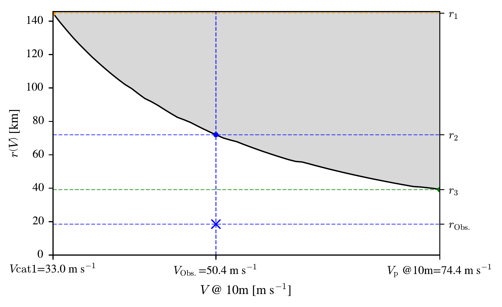
These three metrics together allow us to explore the trade-off between size and central windspeed that might be experienced by a tropical cyclone. In Figure 2.2 we look at how the potential size changes for a particular point in Katrina’s trajectory as we change the velocity at the radius of maximum winds, \(V\). The black curve marks the solution of the potential size model. The area above the black curve is colored grey to signal that it is disallowed in the model because the radius of maximum winds, \(r\), is larger than the potential size at that intensity, \(r\left(V\right)\). For this particular point in time, the observation is well within the allowed region, but we will show that there are observations that appear to be in the disallowed region as well, reaching a ‘supersize’ given their observed intensity, primarily through suspected extratropical transition or data quality issues.
To fully explain the potential size model, we first describe how the two components of the model come together (Section Section 2.2.2.2), and then, once motivated, how each component works in detail (Section Sections 2.2.4 and 2.2.3).
2.2.2.2 Finding Potential Size by satisfying CLE15 and W22 Sub-Carnot Engine
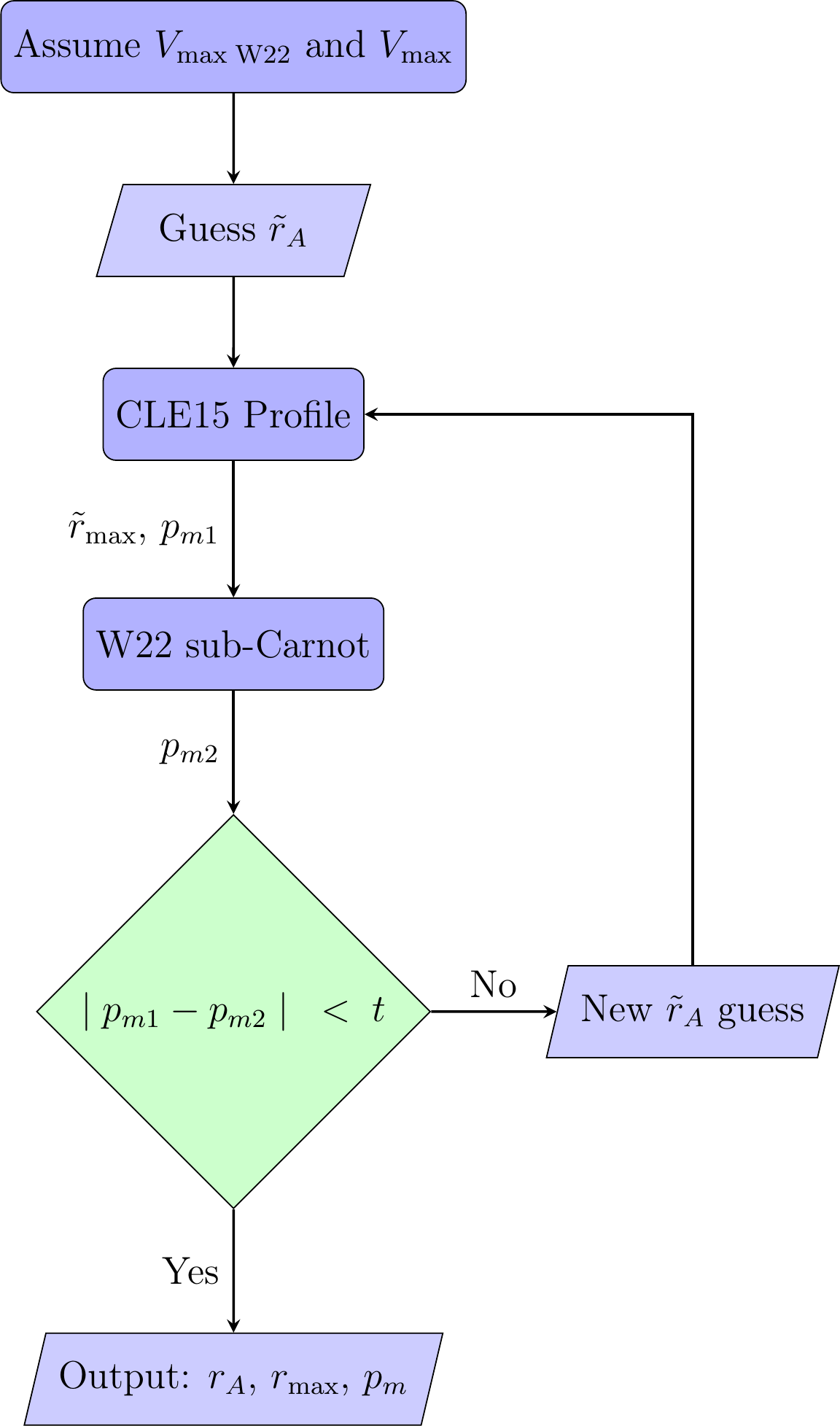
To calculate the potential size, we use the two models in series: the CLE15 dynamic constraint model and the W22 thermodynamic constraint sub-Carnot engine. CLE15 predicts the pressure at the radius of maximum winds from the dynamical wind profile, denoted \(p_{m1}\); W22 predicts the same pressure from the thermodynamic sub-Carnot energy budget, denoted \(p_{m2}\). We vary the outer radius of the TC, \(\tilde{r}_A\), until the two estimates agree to within some tolerance, \(t\), i.e. \(|p_{m1}-p_{m2}|<t\), as shown in Figure 2.3.
In the potential size model there are three key windspeeds to keep track of. The maximum wind speed at 10m, \(V\), the maximum wind speed at the gradient level (the altitude, typically \(\sim\)1 km, at which the Coriolis, centrifugal, and pressure-gradient forces balance above the turbulent surface friction layer (Kepert and Wang 2001)) for the CLE15 profile, \(V_{gm}\), and an enhanced supergradient wind speed for the W22 sub-Carnot engine, \(V_{\mathrm{max\; W22}}\). These are related by the equations,
\[\begin{align} V_{gm} &= \frac{V}{V_{\text{reduc}}},\\ V_{\text{max\; W22}} &= \gamma_{sg} V_{gm}, \end{align}\](2.37) where \(V_{\text{reduc}}=0.8\) is the standard velocity reduction parameter from the gradient wind level to the 10m wind level (see e.g. Gilford 2021), and \(\gamma_{sg}=1.2\) is the supergradient factor of how much higher the wind is assumed to be than the gradient wind at the radius of maximum wind for the W22 sub-Carnot engine. D. Wang et al. (2022) justifies using a supergradient factor for the wind for the W22 sub-Carnot engine based on the observation that TCs have been observed to exceed the gradient wind balance. Also, as discussed in Section Section 2.2.3, the W22 sub-Carnot engine evaluates the specific kinetic energy of the parcel at the radius of maximum winds which should include radial and tangential components, justifying a higher value than the gradient level windspeed for the CLE15 model, \(V_{gm}\).
The CLE15 dynamic constraint depends on the background sea level pressure, \(p_A\), and density, \(\rho_A\), the lower-troposphere subsidence velocity in the subsidence region \(w_{\mathrm{cool}}=0.002 \text{ m s}^{-1}=2\times10^{-3} \text{ m s}^{-1}\), the surface drag coefficient \(C_D=0.0015=1.5\times10^{-3}\) and the surface enthalpy exchange coefficient \(C_k=0.9\times C_D = 1.35\times10^{-3}\) (to be consistent with potential intensity calculation), the Coriolis parameter, \(f\), at that latitude, the gradient level maximum windspeed \(V_{gm}\), and the outer radius, \(\tilde{r}_A\). This leads to a prediction of the pressure at the radius of maximum winds, \(p_{m1}\), and the radius of maximum winds, \(r_{\mathrm{max}}\), \[\begin{equation} \mathrm{CLE15}\left(V_{\text{max}}, \rho_A, p_A, w_{\mathrm{cool}}, f, C_D, C_k; \tilde{r}_A\right) = \left(p_{m1}, \tilde{r}_{\mathrm{max}}\right). \end{equation}\](2.38) The prediction of the pressure, \(p_{m1}\), is made assuming that the gradient wind of the CLE15 profile, \(\hat{V}\left(\hat{r}\right)\), is in cyclogeostrophic balance, and that the air density is calculated that it is an isothermal ideal gas so that the pressure profile is, \[\begin{equation} p\left(\hat{r}\right) = p_A \exp\left(- \frac{\rho_A}{p_A}\int^{\tilde{r}_A}_{\hat{r}} \left(f V\left(\tilde{r}\right)+ \frac{\hat{V}^2\left(\tilde{r}\right)}{\tilde{r}}\right)d\tilde{r}\right), \end{equation}\](2.39) and \(p_{m1}=p\left(r_{\mathrm{max}}\right)\).
The W22 sub-Carnot engine model takes the surface and outflow temperatures, \(T_n\) and \(T_o\)10, the background sea level pressure, \(p_A\), the environmental relative humidity, \(\mathcal{H}_e\), the efficiency relative to the Carnot cycle, \(\eta=\frac{1}{2}\), the lift parametrisation, \(\beta_l=\frac{5}{4}\), the Coriolis parameter, \(f\), the assumed maximum velocity for the sub-Carnot engine which is assumed to be some constant value above the gradient wind value assumed in the CLE15 model, \(V_{\mathrm{max\; W22}}=\gamma_{\mathrm{sg}}V_{gm}\), and the radius of maximum winds, \({\tilde{r}_\mathrm{max}}\), from CLE1511, and the radius of outer winds, \(\tilde{r}_A\), \[\begin{equation} \mathrm{W22}\left(T_n, T_o, p_A, \eta, f, \mathcal{H}_e, V_{\mathrm{max\; W22}}, \beta_l; \tilde{r}_{\mathrm{max}}, \tilde{r}_A\right) = p_{m2}. \end{equation}\](2.40) To converge on a final value of the outer radius, \(r_A\), where \(|p_{m1}-p_{m2}|<t\) then we can change \(\tilde{r}_A\) using the bisection algorithm. We call the final outer radius, \(r_A\), the potential outer size, and the final radius of maximum winds, \(r_{\mathrm{max}}\), the potential inner size.
Figure 2.4 shows a single solution of the potential size calculation summarised in Figure 2.3. The solution marked as a cross is where the two models produce pressures at the radius of maximum windspeed, \(p_{m1}\) and \(p_{m2}\), are within some threshold value, \(t\), of one another (taken arbitrarily as 1 Pa). These two curves are expected to cross because the energetic constraints of the W22 sub-Carnot engine would reduce the central pressure deficit with higher \(r_A\), and the dynamic constraints of the CLE15 radial profile would increase the central pressure deficit with higher \(r_A\). We find the intersection by using the bisection method for simplicity, and because there was not an obvious way of calculating the gradient of pressure deficit by change in outer radius, \(\frac{dp_{m2}}{d r_A}\), for the Chavas et al. (2015) radial profile.
To demonstrate that our method matches D. Wang et al. (2022), Figure 2.4 shows both the data extracted from D. Wang et al. (2022)’s Figure 4a using the WebPlotDigitizer software, and our solution, which is marked as a plus. The small difference between the two is plausibly due either to small differences in the implementation of the CLE15 profile, the numerical integration of the pressure profile, or some combination of both.
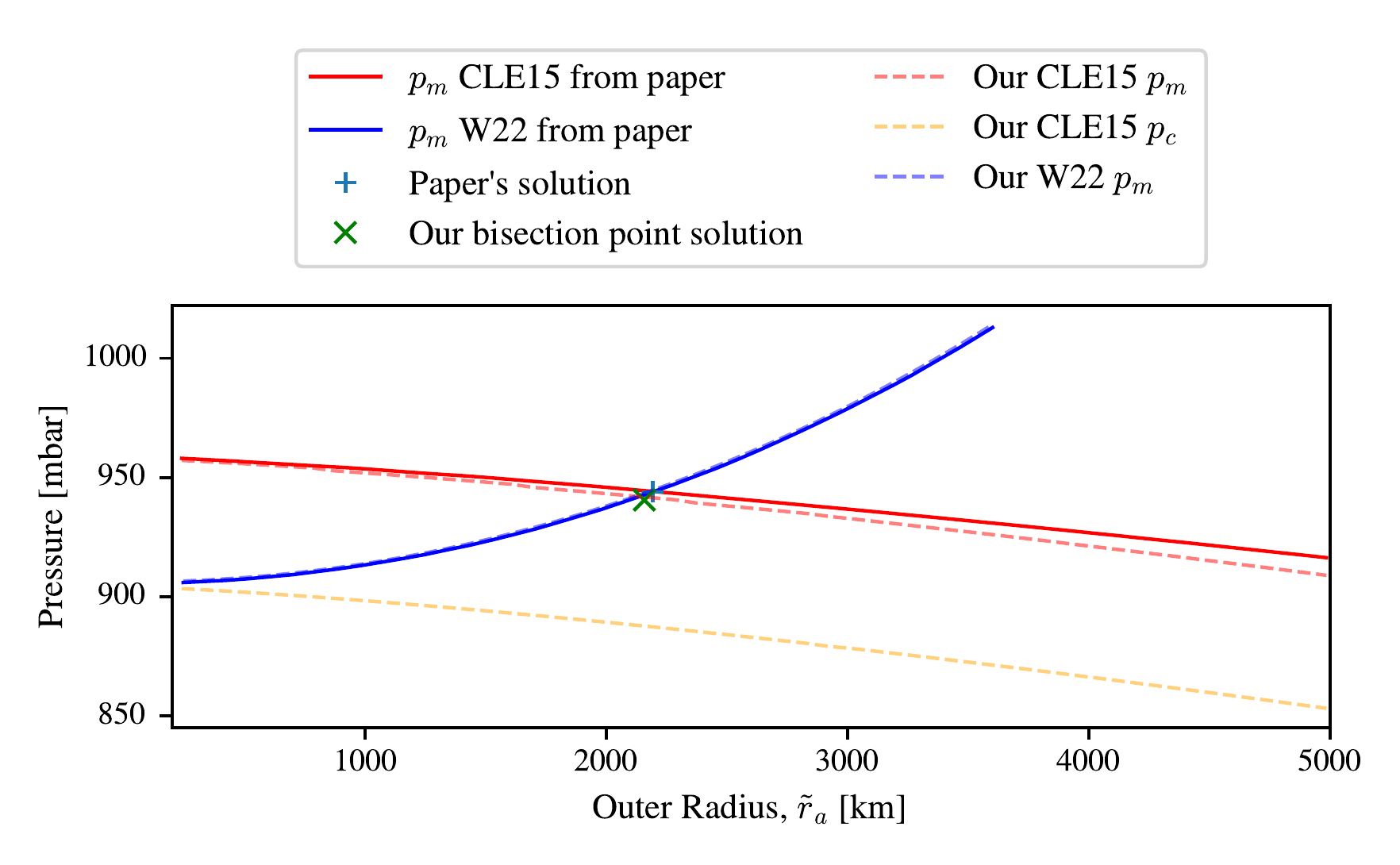
scipy.integrate. The pressure from the CLE15 profile at the
maximum winds is slightly lower in our solution than theirs, which may
be caused by our choice of integration method, or that they used a
higher (unreported) density. \(p_c\) is
the central pressure of the TC in the CLE15 model which is roughly a
constant 50 mbar lower than the pressure at the radius of maximum winds,
\(p_m\) or \(p_B\), for this example.2.2.3 The energetic assumption: The W22 sub-Carnot engine
As with potential intensity, we imagine a thermodynamic cycle running between the sea surface and the upper atmosphere (see Figure 2.6)12. Instead of assuming the thermodynamic cycle is a Carnot engine as in potential intensity Section Section 2.2.1.2, forming a rectangle in \(T-s\) space, we instead assume that it forms a triangle in \(T-s\) space, see Figure 2.7, which leads to a thermodynamic efficiency relative to the Carnot engine, \(\eta\), of precisely 0.5 (D. Wang et al. 2022). This follows geometrically: the work done by any cycle equals the area enclosed in \(T\)-\(s\) space, and the W22 triangle, with the isothermal inflow (A–B at temperature \(T_n\)) as its base and apex at the outflow temperature \(T_o\), has exactly half the area of the Carnot rectangle with the same base \(\Delta s\) and height \(T_n - T_o\). Note that this factor of \(\frac{1}{2}\) is specific to this particular triangular arrangement; a differently shaped cycle would not generally give \(\eta = \frac{1}{2}\eta_\mathrm{Carnot}\). We assume a similar cycle diagram, but add in an additional point called \(A^{\prime}\) where the air parcel reaches the top of the boundary layer (Figure 2.6). At this point, we assume that the air parcel is completely unsaturated and reaches the environmental surface relative humidity at the surface at point \(A\). An additional difference compared to Emanuel (1986) is that instead of assuming that the isothermal inflow’s constant temperature, is at the sea surface temperature, \(T_s\), we instead assume that it is at the near surface air temperature, \(T_n\). To enable calculation, we assume a standard parameterization of \(T_n = T_{s} - 1\text{K}\).
We first start with the moist Bernoulli equation, which is the generalised energy conservation law for a moist air parcel accounting for kinetic energy, work done by pressure, frictional dissipation, and changes in potential energy due to rainout (D. Wang et al. 2022). This can be written as \[\begin{equation} \underbrace{d \left[\left(1 + q_t\right)\frac{1}{2}V_t^2\right]}_{\text{Change in kinetic energy}} = - \underbrace{\alpha_d dp}_{\text{Volume work}} + \underbrace{\vec{F}\cdot d\vec{l}}_{\text{Work against friction}} + \underbrace{\phi dq_t}_{\text{Rain out losses}} - \underbrace{d\left[\left(1+q_t\right)\phi\right]}_{\text{Change in potential energy of parcel}}, \end{equation}\](2.41) where \(q_t\) is the total specific humidity, \(\alpha_d\) is the specific volume of dry air, \(dp\) is the change in pressure, \(\vec{F}\) is the force per unit mass of dry air, \(d \vec{l}\) is the change in position, \(\phi=g z\) is the specific gravitational potential, which is the gravitational acceleration, \(g\), times the height \(z\), \(dq_t\) is the change in total specific humidity, and \(V_t\) is the total magnitude of the wind speed at each point in the cycle. The factor \((1+q_t)\) in the kinetic energy term accounts for the fact that the parcel carries suspended liquid water, so the total moving mass per unit dry-air mass is \((1+q_t)\); without condensate the factor would be unity.
We include the effect of the different species of water by including them in the expression for the specific Gibbs energy change of a parcel (D. Wang et al. 2022). The dry volume work term \(\alpha_d dp\) arises because the standard thermodynamic identity \(dh = Tds + \alpha\, dp\) applies to the dry-air component alone when moisture contributions are separated into the Gibbs terms \(\sum g_w dq_w\), \[\begin{equation} dg = \underbrace{dh}_{\text{Enthalpy change}} - \underbrace{\alpha_d dp}_{\text{Dry volume work}} = \underbrace{Tds}_{\text{Reversible heat transfer}} + \underbrace{\sum g_w dq_w}_{\text{Gibbs free energy of water species}}, \end{equation}\](2.42) where \(dh\) is the change in specific enthalpy, \(\alpha_d\) is the specific volume of dry air, \(dp\) is the change in pressure, \(T\) is the temperature, \(ds\) is the change in specific entropy, \(g_w\) is the specific enthalpy of water species \(w\) and \(dq_w\) is the change in specific humidity of water species \(w \in \left\{v, l, q \right\}\) for vapour liquid or gas. Rearranging this we can write the change in terms \[\begin{equation} \alpha_d dp = Tds + \sum g_w dq_w - dh. \end{equation}\](2.43) We can then simplify the final two terms in Equation (2.41) to become \[\begin{equation} \phi dq_t - d\left[\left(1+q_t\right)\phi\right] = - (1 + q_t) d\phi. \end{equation}\](2.44)
Substituting both of these terms (Equations Equation (2.43) & Equation (2.44)) into Equation (2.41) we find \[\begin{equation} d\left[\left(1 + q_t\right)\frac{1}{2}V_t^2\right] = dh - T ds - \sum g_w dq_w + \vec{F}\cdot d\vec{l} - (1 + q_t) d\phi. \end{equation}\](2.45)
We then integrate this whole expression over the closed cycle, and two of the terms are zero, firstly, \[\begin{equation} \oint d\left[\left(1 + q_t\right)\frac{1}{2}V_t^2\right] = 0 \end{equation}\](2.46) because specific kinetic energy is a state variable, and the cycle is closed. And the same is true for the enthalpy change, which is also a state variable, so that \[\begin{equation} \oint dh = 0. \end{equation}\](2.47)
Integrating the potential energy term gives us \[\begin{equation} \oint \underbrace{(1 + q_t)}_{\text{Specific mass of parcel}} d\phi = \oint q_t d\phi = \oint g q_t dz, \end{equation}\](2.48) because the dry mass of the air is constant over a cycle, and so the only net work done against gravity is for the transport of water, and we can change variables using \(d\phi = g dz\).
Substituting these terms into the loop integral of Equation (2.45) together we can get to the simplified terms \[\begin{align} \oint T ds & + \oint\sum g_w dq_w &=& \oint \vec{F}\cdot d\vec{l} & + \oint q_t d\phi, \\ Q_{s} & + Q_{\mathrm{Gibbs}} &=& W_{\mathrm{PBL}} + W_{\mathrm{Outflow}} & + W_p. \end{align}\](2.49) Where \(Q_s\) is the reversible heat transfer, \(Q_{\mathrm{Gibbs}}\) is the Gibbs free energy change of the water species, \(W_{\mathrm{PBL}}\) is the work done against the planetary boundary layer, \(W_{\mathrm{Outflow}}\) is the work done in the outflow, and \(W_p\) is the work done against gravity from the lifting of water species.
We then assume a parameterization of the work done against gravity, as a constant fraction of the work done in the boundary layer, \(W_{\mathrm{PBL}}\), and in the outflow, \(W_{\mathrm{Outflow}}\), so that, \[\begin{equation} W_{p} = (\beta_l -1)\left(W_{\mathrm{PBL}} + W_{\mathrm{Outflow}}\right), \end{equation}\](2.50) where \(\beta_l=5/4\) is the lift parametrisation, a free parameter of D. Wang et al. (2022). With \(\beta_l=5/4\), the factor \((\beta_l-1)=1/4\) means the work done lifting water equals one quarter of the (PBL + outflow) work, or equivalently one fifth of the total work done by the cycle (since total work \(= \beta_l(W_\mathrm{PBL}+W_\mathrm{Outflow})\), so \(W_p/W_\mathrm{total} = (1/4)/(5/4) = 1/5\)). D. Wang et al. (2022) show that the results are not strongly sensitive to the precise value of \(\beta_l\), and we retain \(\beta_l=5/4\) throughout. This simplifies Equation (2.49) to, \[\begin{align} Q_s + Q_{\mathrm{Gibbs}} & = \beta_l \left(W_{\mathrm{PBL}} + W_{\mathrm{Outflow}}\right). \end{align}\](2.51)
The work done against the planetary boundary layer is \[\begin{align} W_{\mathrm{PBL}} &= \int^{B}_{A'} - \vec{F} \cdot d\vec{l} \quad \text{ which then using the Bernoulli Section~\ref{pips:eq:bernoulli} becomes}\\ &= \underbrace{\int^{B}_{A'} - \alpha_d dp}_{\text{Volume work term}} + \int ^{B}_{A'}-d\underbrace{\left[(1+q_t)\frac{1}{2}\left|\vec{V}\right|^2\right]}_{\text{Change in kinetic energy of parcel}}\\ & \approx R T_n \ln \frac{p_{dA}}{p_{dB}} - 1/2 v_{B}^2 \text{ as } q_v \text{ is small and } v_A \approx 0. \end{align}\](2.52) where \(A^{\prime}\) is the top of the boundary layer, and \(B\) is the radius of the TC at the radius of maximum winds. We can ignore the rain out losses and change in potential energy change of the parcel terms from Equation (2.41) because the \(A\) to \(B\) leg is horizontal.
The absolute momentum is defined as \(M = rv + \frac{1}{2}f r^2\), so that \(v = \frac{M}{r} - \frac{fr}{2}\). We assume that the legs B-C and A-D involve no frictional dissipation, and so have constant absolute angular momentum, i.e. \(M_B=M_C\), and \(M_A=M_D\). We use this to rewrite \(W_{\mathrm{Outflow}}\) in terms of the absolute angular momentum at \(B\) and \(A\), \(M_B\) and \(M_A\). \[\begin{align} W_{\mathrm{Outflow}} &= \int^{D}_{C} - \vec{F} \cdot d\vec{l}, \\ &= -\underbrace{\frac{1}{2}(V_{D}^2 - V_{C}^2)}_{\text{Change in kinetic energy}},\\ &= -\frac{1}{2}\left[\frac{M_D^2}{r_D^2} - \frac{M_C^2}{r_C^2} - fM_D + fM_C + \frac{f^2 r_D^2}{4} - \frac{f^2r_C^2}{4} \right] \quad \text{ and then assume } r_D=r_C,\\ &= - \frac{1}{2} \left[\frac{M_D^2 - M_C^2}{r_C^2} - f\left(M_D - M_C\right)\right] \quad \text{and assume } M_D=M_A \text{, and } M_C = M_B,\\ &= - \frac{1}{2} \left[\frac{M_A^2 - M_B^2}{r_C^2} - f\left(M_A - M_B\right)\right] \quad \text{and assume } v_A = 0 \text{ so } M_A = \frac{1}{2}fr_A^2,\\ &= - \frac{1}{2} \left[\frac{M_A^2 - M_B^2}{r_C^2} - \frac{f^2 r_A^2}{2} + f M_B\right],\\ &= \frac{1}{4}f^2 r_A^2 - \frac{1}{2} f M_B - \frac{1}{2}\frac{M_A^2 - M_B^2}{r_C^2},\\ &= \frac{1}{4}f^2 r_A^2 - \frac{1}{2} f M_B \quad \text{when } r_C\to +\infty. \end{align}\](2.53)
We use this final form assuming that the dissipation radius \(r_D = r_C \to +\infty\). Physically, this is reasonable because the kinetic energy of the outflow, \(\frac{1}{2}V^2 \propto r^{-2}\), becomes negligible at large radii, so extending the dissipation region to infinity introduces little error. D. Wang et al. (2022) also explore the alternative \(r_D=\frac{5}{4} r_A\), and the results are not strongly sensitive to this choice.
The new specific entropy of a parcel in D. Wang et al. (2022) is given by \[\begin{equation} s = \underbrace{c_{pd}\ln\left(\frac{T}{T_{\text{Trip}}}\right)}_{\text{Temperature contribution}} + \underbrace{q_v \frac{L_v}{T}}_{\text{Latent heat contribution}} - \underbrace{R \ln\left(\frac{p_d}{p_o}\right)}_{\text{Dry pressure contribution}} - \underbrace{q_v R_v \ln\left(\mathcal{H}\right)}_{\text{Water vapour pressure contribution}}, \end{equation}\](2.54) where \(c_{pd}\) is the specific heat capacity of dry air at constant pressure, \(T\) is the temperature, \(T_{\text{Trip}}\) is the temperature at the triple point of water, \(R\) is the specific gas constant for dry air, \(p_d\) is the partial pressure of dry air, \(p_o\) is a reference pressure (1000 hPa), \(q_v\) is the specific humidity of water vapour, \(L_v\) is the latent heat of vaporization, \(R_v\) is the specific gas constant for water vapour and \(\mathcal{H}\) is the relative humidity. The main difference to the previous entropy Equation (2.7) is the addition of the water vapour pressure term as distinct from the dry air pressure term.
The sensible heat input, \(Q_s\), is then \[\begin{align} Q_s & = \oint T ds, \\ & = \int^{B}_{A'} T_n ds + \int^{D}_{C} T_{0} ds, \\ & = \eta \epsilon_C \int ^{B}_{A'} T_n ds, \\ & \text{ assuming that the thermodynamic cycle is a constant fraction } \eta \text{ of the Carnot efficiency } \epsilon_C, \notag\\ & = \eta \epsilon_C T_n \left(s_B - s_{A'}\right), \\ & = \eta \epsilon_C T_n \left( \frac{L_v}{T_n}\left(q_{vB}- q_{vA'}\right) + R\ln{\frac{p_{dA}}{p_{dB}}} - R_v\left(q_{vB}\ln{\mathcal{H}_B} - q_{vA'}\ln{\mathcal{H}_A'}\right)\right),\\ & \approx \eta \epsilon_C \left(L_v q_{vB} + R T_n \ln{\frac{p_{dA}}{p_{dB}}}\right), \end{align}\](2.55) where we assume that \(T_n \approx T_{A'} \approx T_B\), \(q_{vA'} \approx 0\) as the air is unsaturated at the top of the boundary layer (\(A^{\prime}\)), and \(\mathcal{H}_B \approx 1\) as the air is saturated at point \(B\). \(p_{dA}\) is the partial pressure of dry air at point \(A^{\prime}\), and \(p_{dB}\) is the partial pressure of dry air at point \(B\). The Carnot efficiency is defined as \(\epsilon_C=\frac{T_n-T_o}{T_n}\).
The specific Gibbs free energy of water vapour can be approximated as (Emanuel 1994; D. Wang et al. 2022), \[\begin{equation} g_v \approx R_v T \left(\ln{q_v} + c_1\right), \end{equation}\](2.56) where \(c_1 = -\ln{e_s^{*}} + \ln{\left(\frac{R_v}{R} \cdot p_{dA}\right)} = - \ln{\left(q_{va}^{*}\right)}\) is a constant at fixed surface pressure and temperature. Physically, \(c_1\) is the negative logarithm of the saturation specific humidity at the surface, \(q_{va}^{*}\), and absorbs the reference-state dependence of the chemical potential; \(e_s^{*}\) is the saturation vapour pressure at the surface temperature, \(T_n\).
We assume that the only significant species in the Gibbs heat input, \(Q_{\mathrm{Gibbs}}\), is water vapour, and that this almost entirely occurs in the inflow from the point of complete desaturation, \(A^{\prime}\), to the point of saturation at the radius of maximum winds, \(B\). This gives us \[\begin{align} Q_{\mathrm{Gibbs}} & = \oint \sum g_w dq_w, \\ & \approx \oint g_v dq_v, \\ & \approx \int^{q_{vB}}_{q_{vA'}} g_v dq_v, \\ & \approx \int^{q_{vB}}_{q_{vA'}} R_V T_n \left(\ln{q_v} + c_1\right) dq_v,\\ & = R_v T_n \left[(c_1-1)q_v + q_{v}\ln{q_v} \right]^{q_{vB}}_{q_{vA'}}, \\ & \approx R_v T_n q_{vB} \left(c_1 - 1 +\ln{q_{vB}} \right), \\ & = R_v T_n q_{vB}\left(\ln{\frac{q_{vB}}{q_{vA}^{*}}} - 1 \right),\\ & = R_v T_n q_{vB}\left(\ln{\frac{p_{dA}}{p_{dB}}} - 1\right). \end{align}\](2.57) Where we assume that \(T_n \approx T_{A'} \approx T_B\), \(q_{vA'} \approx 0\) as the air is unsaturated at the top of the boundary layer, and \(q_{vB} = q^{*}_{vB}\) as the air is saturated at point \(B\). \(p_{dA}\) is the partial pressure of dry air at point \(A^{\prime}\), and \(p_{dB}\) is the partial pressure of dry air at point \(B\). We can also use the approximation that \(q_{vB} \approx \epsilon e_s^{*}/p_{dB}\) where \(\epsilon = R_d/R_v\).
Equation (2.51) then becomes, \[\begin{align} Q_s + Q_{\mathrm{Gibbs}} & = \beta_l \left(W_{\mathrm{PBL}} + W_{\mathrm{Outflow}}\right), \end{align}\](2.58) \[\begin{align} \eta \epsilon_{C} \left(L_v q_{vB} + R T_n \ln{\frac{p_{dA}}{p_{dB}}}\right) + R_v T_n q_{vB}\left(\ln{\frac{p_{dA}}{p_{dB}}} - 1\right) \notag \\ = \beta_l \left(R T_n \ln \frac{p_{dA}}{p_{dB}} - \frac{1}{2} v_{\text{max W22}}^2 + \frac{1}{4}f^2 r_A^2 - \frac{f M_B}{2}\right), \end{align}\](2.59) through substituting in terms from equations Equation (2.57), Equation (2.55), Equation (2.52), & Equation (2.53).
We then use the substitution for \(q_{vB}\) using the fact that the air is saturated at point \(B\), so that \[\begin{equation} q_{vB} = \frac{R e_s^{*}}{R_v p_{dB}} = \frac{R e_s^{*}}{R_v p_{dA}} \frac{p_{dA}}{p_{dB}}, \end{equation}\](2.60) where \(e_s^{*}\) is the saturation vapour pressure at temperature \(T_n\), \(p_{dA}\) is the partial pressure of dry air at point \(A\), and \(p_{dB}\) is the partial pressure of dry air at point \(B\).
We can also define a variable, \(y\), \[\begin{equation} y = \frac{p_{dA}}{p_{dB}}, \end{equation}\](2.61) to rewrite the equation as, \[\begin{equation} y = \exp\left(E y + F y \ln{y} + G\right), \end{equation}\](2.62) where \[\begin{align} E &= \frac{e_s^{*}}{p_{dA}}\frac{\eta \epsilon_{C}L_v/R_v -T_n }{\left(\beta_l - \eta \epsilon_C\right)T_n}, \\ F &= \frac{e_s^{*}}{p_{dA} \left(\beta_l - \eta \epsilon_C\right)}, \\ G &= \frac{\beta_l}{\left(\beta_l - \eta \epsilon_C\right) R T_n } \left(-\frac{1}{2}V_{\mathrm{max\; W22}}^2 + \frac{1}{4}f^2r_A^2 -fM_B \right). \end{align}\](2.63)
We can solve this transcendental equation through bisection if we assume some values for \(r_A\) and \(V_{\mathrm{max\; W22}}\). The values for the other parameters can be taken from the environment, and we keep \(\eta=0.5\) and \(\beta_l=5/4\) as in D. Wang et al. (2022). The solution to this equation gives us the pressure at the radius of maximum winds, given the environmental input parameters and the assumed \(r_A\) and \(V_{\text{max W22}}\). The term \(M_B\) is the absolute angular momentum at the radius of maximum winds, which can be calculated as \(M_B = r_{\text{max}} V_{\text{max\; W22}} + \frac{1}{2} f r_{\text{max}}^2\), where \(r_{\text{max}}\) is the radius of maximum winds. This brings in an additional parameter \(r_{\mathrm{max}}\) which we can take from the CLE15 (Chavas et al. 2015) model, implying that we run the CLE15 model for the same conditions first.
2.2.3.1 Assumptions and limitations
The key assumptions of the W22 sub-Carnot engine are:
The TC is in steady state.
The TC is axisymmetric.
We are on the \(f\)-plane.
The thermodynamic efficiency of the sub-Carnot cycle is a constant fraction, \(\eta=0.5\), of the Carnot cycle.
There are no diffusive losses of kinetic energy.
Work done lifting water is a constant factor \((\beta_l - 1)=\frac{1}{4}\) of the sum of the frictional dissipation in the boundary layer and the frictional dissipation in the outflow.
The leg \(B\)-\(C\) is approximately adiabatic (constant specific entropy \(s\)) and conserves absolute angular momentum.
The leg \(D\)-\(A^{\prime}\) also has constant absolute angular momentum \(M\), but is not adiabatic.
The outflow cooling leg \(C\)-\(D\) starts at the outflow temperature \(T_o\), and reduces absolute angular momentum from \(M_B\) to \(M_A\). We additionally assume that \(r_C = r_D \to \infty\) to simplify this.
We assume the entire Gibbs energy contribution occurs in the inflow, and ignore the contributions of ice and liquid water.
We assume that the air is saturated at the radius of maximum winds (point \(B\)), and unsaturated at the top of the boundary layer (point \(A^{\prime}\)).
We assume that the air is an ideal gas, and that the atmosphere is in hydrostatic balance.
2.2.4 The Dynamic Assumption: The CLE15 radial profile
2.2.4.1 Motivation
In order to use TC potential size, we had to use the CLE15 profile as the dynamic constraint. This profile is also used in later Chapters 3 and 4 as the wind profile to force the numerical storm surge model.
TCs exhibit a characteristic radial structure in their wind and pressure fields, with winds rising from near zero at the centre to a peak at radius of maximum winds, \(r_{\mathrm{max}}\), near the eyewall and then decaying outward to near zero at the storm’s outermost extent. Understanding and modelling this radial structure is critical for predicting storm hazards and for theoretical insight into cyclone dynamics. Traditional empirical wind profiles (for example Holland’s model Holland 1980; Holland et al. 2010) can fit observed winds but lack a direct physical basis. Chavas et al. (2015) developed a physically based analytic model for the complete low-level radial wind structure of an axisymmetric steady state TC by uniting an inner core solution and an outer region solution from prior theory. The model captures known behaviours, such as an anticorrelation between intensity and \(r_{\mathrm{max}}\) (inner core contraction with strengthening), and the relative independence of outer circulation size.
2.2.4.2 Emanuel (2004) outer wind solution (E04)
A cornerstone of the model is the theoretically motivated outer region wind solution due to Emanuel (2004). Emanuel (2004) model the dry, rain-free outer circulation of a TC: the region beyond the moist convective inner core (eyewall), where air subsides rather than rises. In this outer region, air descends slowly from the tropopause in approximate radiative–convective equilibrium with a radiative cooling rate \(W_{\mathrm{cool}}\) of order a few \(\mathrm{mm}\,\mathrm{s^{-1}}\) and spirals cyclonically near the surface under frictional drag. Emanuel (2004) assumed an axisymmetric steady state storm and applied angular momentum and mass continuity at the top of the boundary layer. The key assumption is that downward mass flux induced by radiative cooling balances upward Ekman suction driven by surface friction in the outer circulation.
Let \(M(r)\) be the absolute angular momentum per unit mass, \[\begin{equation} M(r)=r\,V(r)+\tfrac12 f r^{2}, \end{equation}\](2.64) where \(V(r)\) is the azimuthal wind and \(f\) is the Coriolis parameter (assumed constant, i.e. on an \(f\)-plane). In the boundary layer the radial convergence of momentum due to surface stress and the vertical advection of momentum due to subsidence determine the radial gradient of \(M\). Emanuel (2004) showed that this balance yields \[\begin{equation} \frac{\mathrm{d}M}{\mathrm{d}r}=\frac{2\,C_d}{W_{\mathrm{cool}}}\,\frac{\bigl(r\,V(r)\bigr)^{2}}{r_A^{2}-r^{2}}, \end{equation}\](2.65) where \(C_d\) is the surface drag coefficient and \(r_A\) is the radius of vanishing wind. Equation (2.65) must be solved numerically. Emanuel (2004) recast it nondimensionally via \(\tilde r=r/r_A\) and \(\tilde M=M/M_0\) with \(M_0=\tfrac12 f r_A^{2}\), \[\begin{equation} \frac{\mathrm{d}\tilde M}{\mathrm{d}\tilde r}=\gamma\,\frac{\tilde M-\tilde r^{2}}{1-\tilde r^{2}}, \end{equation}\](2.66)
in which \(\gamma=f\,r_A\,C_d/W_{\mathrm{cool}}\). Physically, \(\gamma\) measures the ratio of frictional momentum extraction to radiative subsidence: a larger Coriolis parameter \(f\) anchors more angular momentum to the planetary rotation; larger \(r_A\) increases the angular momentum reservoir at the storm boundary; larger \(C_d\) amplifies frictional spin-up; and smaller \(W_{\mathrm{cool}}\) reduces the stabilising subsidence that suppresses the outer circulation. The boundary condition is \(\tilde M(1)=1\). Because \(\tilde M>\tilde r^{2}\) everywhere inside the outer region, Equation (2.66) shows that \(\mathrm{d}\tilde M/\mathrm{d}\tilde r\) is positive and proportional to \(\gamma\): larger \(\gamma\) therefore makes the angular momentum profile rise more steeply with radius, meaning \(M\) reaches its boundary value over a shorter normalised distance; i.e. the vortex is spatially broader (larger \(r_A\) for a given \(V_{\mathrm{max}}\)), not that winds decay more slowly in time. Conversely, smaller \(\gamma\) produces a tighter vortex with winds that fall off rapidly outward.
2.2.4.3 Inner core solution (ER11)
The inner core wind structure is determined by moist thermodynamics and rapid ascent in the eyewall. Emanuel and Rotunno (2011) revisited potential intensity theory by allowing the outflow temperature \(T_{\mathrm{out}}(r)\) to vary radially, yielding an approximate analytic solution for \(M(r)\) inside the eyewall. Expressed in the form adopted by Chavas et al. (2015), \[\begin{equation} \left(\frac{M(r)}{M_m}\right)^{\tfrac{2\,C_h}{C_d}}= \frac{2\,(r/r_{\mathrm{max}})^{2}}{2-\tfrac{C_h}{C_d}+\tfrac{C_h}{C_d}\,(r/r_{\mathrm{max}})^{2}}, \end{equation}\](2.67) where \(C_h\) is the surface enthalpy exchange coefficient, \(M_m\equiv M(r_{\mathrm{max}})=r_{\mathrm{max}}\,V_{gm}+\tfrac12 f r_{\mathrm{max}}^{2}\) and \(V_{gm}\) is the gradient-level maximum wind speed. Larger \(C_h/C_d\) gives a steeper eyewall peak.
2.2.4.4 Composite wind field
Chavas et al. (2015) merge the inner solution Equation (2.67) with the outer solution Equation (2.65). They define a merge radius \(r_{\mathrm{merge}}\) where the two angular momentum curves intersect. Continuity requires \[\begin{equation} M_{\text{inner}}(r_{\mathrm{merge}})=M_{\text{outer}}(r_{\mathrm{merge}}). \end{equation}\](2.68) Additionally, we also require the first derivative of \(M\) to be continuous at \(r_{\mathrm{merge}}\), which is a consequence of the boundary layer gradient balance. This gives a second condition \[\begin{equation} \frac{\mathrm{d}M_{\text{inner}}}{\mathrm{d}r}(r_{\mathrm{merge}})=\frac{\mathrm{d}M_{\text{outer}}}{\mathrm{d}r}(r_{\mathrm{merge}}). \end{equation}\](2.69) The two conditions yield a system of two equations in the two unknowns \(r_{\mathrm{merge}}\) and \(M(r_{\mathrm{merge}})\). We can assume that we know either \(r_\mathrm{max}\), \(r_{\mathrm{merge}}\), or \(r_A\), and this will determine the other two, assuming we already knew \(C_h/C_d\), \(W_{\mathrm{cool}}\), \(V_{gm}\) and \(f\).
For given \(V_{gm}\), \(r_{\mathrm{max}}\), \(f\), \(C_h/C_d\) and \(W_{\mathrm{cool}}\) this condition determines \(r_A\) (or vice versa). \[\begin{equation} V(r)=\frac{M(r)-\tfrac12 f r^{2}}{r}, \end{equation}\](2.70) with \(M(r)\) from Equation (2.67) for \(0\le r\le r_{\mathrm{merge}}\) and from Equation (2.65) for \(r_{\mathrm{merge}}\le r\le r_A\).
To obtain the pressure profile \(p(r)\) from the wind field, Chavas et al. (2015) integrate the gradient-wind balance radially inward, assuming an isothermal temperature profile at the near-surface temperature \(T_n\), so that the air density is \(\rho = p / (R\,T_n)\). This gives an exponential pressure profile and is a standard simplification for the outer region, where horizontal temperature variations are small; the approximation introduces modest errors in the central pressure \(p_{m1}\) for very intense storms where the inner-core temperature structure departs significantly from isothermal.
Figure 2.8 shows an example of the wind and pressure profiles from the CLE15 model. The inner solution (green) is from ER11 and the outer solution (orange) is from E04. The merge radius \(r_{\mathrm{merge}}\) is where the two solutions meet. The inner solution is given by Equation (2.67) and the outer solution by Equation (2.66). The non-dimensional angular momentum, \(M/M_A\), as a function of non-dimensional radius, \(r/r_A\), for the same example is shown in Figure 2.9.
2.2.4.5 Assumptions and limitations
The key assumptions are:
Axisymmetry and steady state.
Boundary layer gradient balance.
Slantwise moist neutrality in the eyewall.
Fixed \(C_h/C_d\) and \(W_{\mathrm{cool}}\).
No active outer rainbands or secondary eyewalls.
Smooth continuity of \(M(r)\) at \(r_{\mathrm{merge}}\) (Match \(M\) and \(M^{\prime}\) at \(r_{\mathrm{merge}}\)).
2.2.4.6 Observational validation and applications
Chavas et al. (2015) compare their wind profiles with aircraft and surface analyses and find good agreement, especially in the outer region. The model is now used in hazard assessment, size climatology and climate change studies because it converts a few basic storm parameters into a full wind field (S. Wang et al. 2022; Chaigneau et al. 2024).
2.3 Methodology
2.3.1 Data
2.3.1.1 IBTrACS Data
In order to compare the potential size and intensity against
observations, we use the International Best Track Archive for Climate
Stewardship (IBTrACS) dataset (we use v04r01 Knapp et al. 2018). We take data only from
1980 to the end of 2024, as it is more reliable due to the ability to
assimilate satellite data. The data is available at https://www.ncdc.noaa.gov/ibtracs/ with filename
IBTrACS.since1980.v04r01.nc. We principally use the central
latitude and central longitude of the TC, the time of the observation,
the observed maximum wind speed (wmo_wind), and the radius
of maximum winds (usa_rmw, mainly available in the North
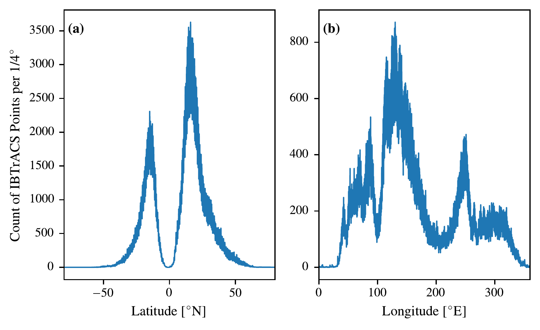
Atlantic and sometimes in the Pacific). Figure 2.10 shows the histogram
of reported points from IBTrACS storms over latitude and longitude from
1980 to 2024.
2.3.1.2 ERA5 Data
We use monthly-mean ERA5 data (Hersbach et al. 2020) (i.e. fields averaged over each calendar month) from 1980 to 2024 to calculate the potential intensity of TCs. The data is available at https://www.ecmwf.int/en/forecasts/datasets/reanalysis-datasets/era5. We choose to use monthly-mean data because the time-averaging means it is not contaminated by the TC’s own cold wake or thermodynamic imprint on the atmosphere. The ERA5 data is available on a 0.25\(^{\circ}\) degree rectilinear lon-lat grid. We use the single level variables of sea surface temperature, two metre temperature, two metre dew point temperature, and mean sea level pressure, as well as the atmospheric volume variables of temperature, specific humidity, and geopotential. The single level variables are used to calculate the potential intensity and size, while the atmospheric volume variables are used to calculate the convective available potential energy (CAPE) and the virtual potential temperature.
Relative humidity, \(\mathcal{H}\), is calculated from the 2m temperature \(t_2\) and dew point temperature \(d_2\), through the formula from Alduchov and Eskridge (1996), \[\begin{equation} \mathcal{H} = \frac{\exp\left(\frac{17.625\, d_2}{d_2 + 243.04}\right)}{\exp\left(\frac{17.625\,t_2}{t_2 + 243.04}\right)}. \end{equation}\](2.71) We use the ERA5 data to calculate the potential intensity and size of TCs using the method described in Section Section 2.2.1 and Section Section 2.2.2. When we compare against CMIP6 (Section Section 2.3.1.3), we regrid ERA5 onto the same 0.5\(^{\circ}\) rectilinear grid as the CMIP6 data using CDO (Schulzweida 2023).
| Variable | Units |
|---|---|
| Single Level Variables | |
sea_surface_temperature |
K |
mean_sea_level_pressure |
Pa |
2m_dewpoint_temperature |
K |
2m_temperature |
K |
| Atmospheric Volume Variables | |
temperature |
K |
specific_humidity |
kg/kg |
geopotential |
m\(^2\) s\(^{-2}\) |
2.3.1.3 CMIP6 Data
We use CMIP6 data from the Pangeo catalogue. We use only the historical (to be able to compare to ERA5 etc.) and SSP5-8.5 (the most extreme climate change scenario) experiments. As calculating potential size is currently very computationally expensive, we limit ourselves to only using CESM2, HadGEM3-GC31-MM, and MIROC6 models. These are chosen as they are from different modelling centres and do not reuse the same components for their ocean or atmosphere, and so are somewhat independent. For each we select the first three ensemble members available on Pangeo to give a sense of the spread. We use monthly average data from the Omon Ocean and Amon Atmospheric tables (Table 2.4). We interpolate from the native atmospheric and ocean grids onto a 0.5\(^{\circ}\) rectilinear grid using CDO (Schulzweida 2023) with a bilinear regridding scheme.
Whilst HighResMIP’s higher-resolution data has lower biases, particularly for explicitly modelling tropical cyclones, we view CMIP6 as adequate for our purpose. As the potential size and potential intensity models only rely on broad-scale fields like sea surface temperature and humidity, we believe that the lower-resolution models do not have substantially higher biases in these fields (Moreno-Chamarro et al. 2022), and many biases such as the double-ITCZ cold-tongue bias are present in both (see e.g. Zhou et al. 2022). Pragmatically, the potential size model is also currently very expensive to run, and so calculating the model on lower-resolution data also substantially reduces our compute costs. We think this highlights one of the advantages of using potential intensity and size, as we hope that they are usefully calculable even on the current round of low-resolution climate models.
| Key | Variable | Units |
|---|---|---|
| Atmospheric Volume Variables | ||
ta |
Air temperature, \(T_a\) | K |
hus |
Specific humidity, \(q\) | kg/kg |
| Atmospheric Surface Variables | ||
tas |
2m temperature, \(t_2\) | K |
huss |
2m specific humidity, \(q_2\) | kg/kg |
hurs |
2m relative humidity, \(\mathcal{H}_2\) | % |
psl |
Mean sea level pressure, \(p_A\) | Pa |
| Ocean Surface Variables | ||
tos |
Sea surface temperature, \(T_s\) | K |
| Model | Institution | Members |
|---|---|---|
| CESM2 | National Center for Atmospheric Research (NCAR), US | r4i1p1f1,
r10i1p1f1, r11i1p1f1 |
| HadGEM3-GC31-MM | Met Office Hadley Centre, UK | r1i1p1f3,
r2i1p1f3, r3i1p1f3 |
| MIROC6 | Japan Agency for Marine-Earth Science and Technology (JAMSTEC) | r1i1p1f1,
r2i1p1f1, r3i1p1f1 |
2.3.2 Comparing IBTrACS and Potential Intensity and Size based on ERA5
The track at index \(j\) in the IBTrACS dataset has a sequence of central longitudes \(\mathrm{lon}_{ij}\), central latitudes \(\mathrm{lat}_{ij}\) for each time \(\mathrm{time}_{ij}\) at time index \(i\). The ERA5 monthly dataset from 1980 has indices \((x, y, t)\), where \(x\) and \(y\) are the latitude index and longitude index of the grid point for the grid points longitude \(\mathrm{lon}_{x}\) and latitude \(\mathrm{lat}_{y}\), and \(t\) is the time index for time \(\mathrm{time}_t\). For each track point \(ij\) in IBTrACS, we find the closest ERA5 grid point, by separately minimising the distance between the longitude, latitude and time indices \[\begin{equation} \left(x, y, t\right)^{ij} = \arg \min_{x, y, t}\left(|\mathrm{lon}_{ij} - \mathrm{lon}_{x}|, |\mathrm{lat}_{ij}- \mathrm{lat}_y|, |\mathrm{time}_{ij} - \mathrm{time}_t| \right). \end{equation}\](2.72) We then only keep the sets of indices \((x, y, t)\) that are unique by storing them in a hashmap \[\begin{equation} \left(x, y, t\right) \to u, \end{equation}\](2.73) where \(u\) is the corresponding index for the \(u\)th unique gridpoint. There are a total of 275,598 points for which we have to calculate the potential intensity and size between 1980–2024 (inclusive). Figure 2.11 shows the number of unique points in the ERA5 dataset that correspond to tracks in the IBTrACS dataset as a heatmap across the globe. If the same ERA5 grid point is passed by multiple tracks in the same month, then this will only be counted once, which perhaps leads to Figure 2.11 understating TC activity in the most active regions (North West Pacific and the North East Pacific).
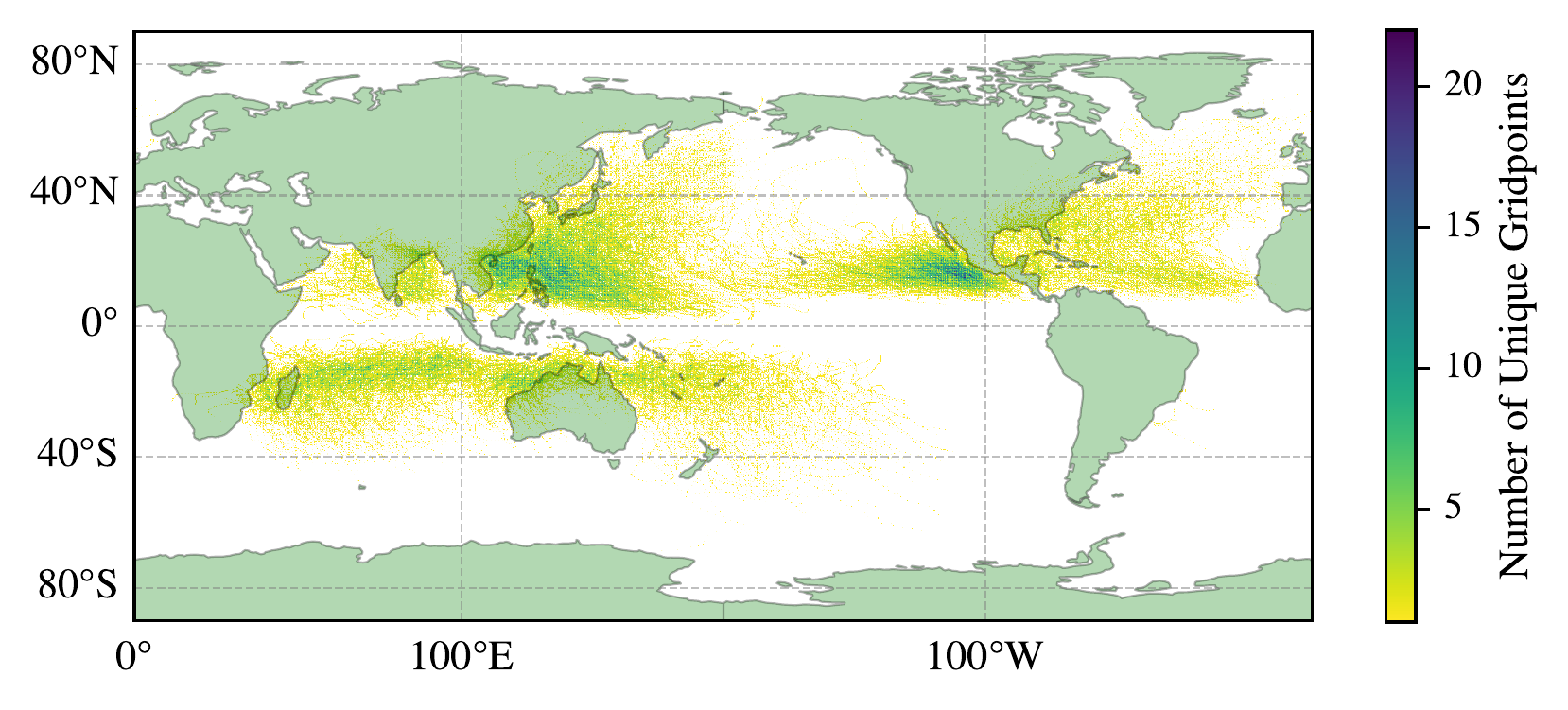
2.4 Results: Comparing Potential Intensity and Potential Inner Sizes to Observations
2.4.1 Property definitions
In order to be able to test the validity of our adaptation of the potential size model, we define the following observed and potential properties for TCs. The observations are:
Observed Maximum Wind Speed (\(V_{\mathrm{Obs.}}\)): The maximum 10-meter wind speed observed in the IBTrACS dataset.
Observed Radius of Maximum Winds (\(r_{\mathrm{Obs.}}\)): The radius of maximum winds observed in the IBTrACS dataset, which is primarily reported by US weather agencies, leading to a geographical bias towards the North Atlantic and North East Pacific basins.
The potential properties, calculated using corresponding ERA5 monthly data, are defined as follows:
Potential Intensity (\(V_p\)@10m): This represents the proposed maximum 10-meter wind speed a tropical cyclone can attain under given environmental conditions, serving as the widely accepted baseline for tropical cyclone intensity (Emanuel 1986; Bister and Emanuel 2002; Gilford 2021).
PI Potential Inner Size (\(r_3\)): The radius of maximum winds, calculated assuming the tropical cyclone has reached its full potential intensity, \(V_p\). This is most relevant for the most intense storms.
Corresponding Potential Inner Size (\(r_2\)): The radius of maximum winds, calculated assuming the tropical cyclone’s intensity is its observed maximum wind speed, \(V_{\mathrm{Obs.}}\). This measure is relevant for all observed storms, providing a proposed maximum size benchmark based on the storm’s actual observed strength.
Category 1 Potential Inner Size (\(r_1\)): The radius of maximum winds, calculated assuming the tropical cyclone’s intensity is at least the minimum threshold for a Category 1 hurricane, 33 at 10m. This measure is particularly useful for less intense storms and helps to isolate the influence of potential size dynamics from variations in potential intensity.
Based on these, we define the observations that exceed our potential models as:
Superintensity: When \(V_{\mathrm{Obs.}} / V_p > 1\) (see e.g. Persing and Montgomery 2003).
Supersize: When \(r_{\mathrm{Obs.}} / r_2 > 1\), a new term.
2.4.2 Example Storm: Hurricane Katrina
In order to show what these potential and observed properties look like for a single storm, we plot Hurricane Katrina (2005) in Figure 2.12. We can see in Figure 2.12(a) and (b) that after its initial landfall in Florida,13 Katrina rapidly intensified over the warm waters of the Gulf of Mexico, peaking at Category 5 intensity, at almost exactly its potential intensity, before making its final landfall as a Category 3 hurricane. The PI potential size, \(r_3\), assuming the storm reached \(V_p\), remained relatively constant and was frequently exceeded by the observed size, \(r_{\mathrm{Obs.}}\) (Figure 2.12(c)), particularly when the observed intensity was significantly below \(V_p\). This is expected, because its definition assumes the storm has reached \(V_p\), and if the storm is less intense than that, the potential size model predicts it can still exhibit a larger observed size than \(r_3\) because their \(r_2 > r_3\). More fundamentally, this reflects an intrinsic prediction of the potential size framework: for a given thermodynamic environment, a storm operating below its potential intensity has a larger theoretical outer circulation; the model predicts that \(r_{\mathrm{max}}\) increases as \(V_{\mathrm{Obs.}}\) decreases toward sub-potential values, so an anti-correlation between intensity and size is built into the framework (Chavas et al. 2017). In contrast, the corresponding potential size \(r_2\), calculated using \(V_{\mathrm{Obs.}}\), generally decreased as the storm intensified. While \(r_{\mathrm{Obs.}}\) was mostly smaller than \(r_2\), a brief period of \(r_{\mathrm{Obs.}} > r_2\) occurred near peak intensity, and was relatively small, well within the observational uncertainty in \(r_{\mathrm{Obs.}}\). Overall, Katrina largely conformed to the expected behavior of potential intensity and size, with its near-attainment of these limits underscoring its extreme nature, but the storm never becomes notably superintense or supersized. Appendix Section Section 2.11.1 contains similar plots for other notable TCs.
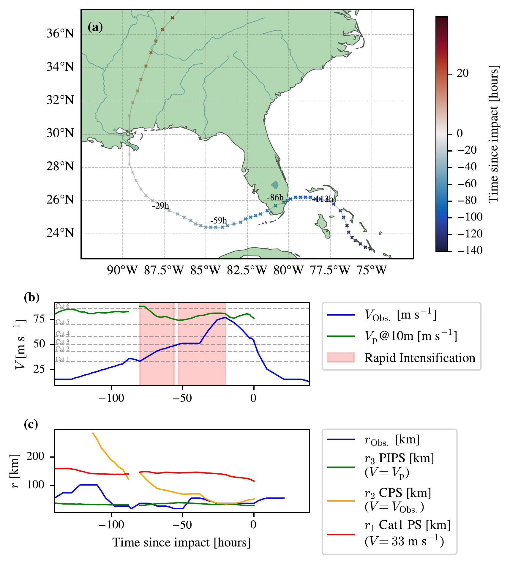
2.4.3 Distributions of Normalized Intensity and Size
To understand the performance of these potential size variables at constraining the observed size and intensity of storms we begin by examining the distributions of normalized intensity (\(V_{\mathrm{Obs.}} / V_p\)) and normalized size (\(r_{\mathrm{Obs.}} / r_x\), where \(r_x\) is one of the potential size measures). To ensure that our analysis focuses on genuinely tropical systems, we at minimum filter the data with the standard filter SF. This filters to include only points where both the potential intensity, \(V_p\), and the observed maximum wind speed \(V_{\mathrm{Obs.}}\) exceed 33 , corresponding to the minimum intensity of a Category 1 hurricane. This threshold helps to exclude some of the weak and/or non-tropical storms where the underlying thermodynamic assumptions for PI and PS apply less well, and its effect is explored in Appendix Section Section 2.12.
We find with this SF filter alone storms often become supersized storms, and so it is necessary to impose additional filters. From investigating particular examples (see Section Section 2.4.4.0.2) we found that many of the supersized storms in the SF dataset were weak, high-latitude, or extratropically transitioning systems, all contexts where the potential size model’s core assumptions (warm-core structure, axisymmetry, and a purely tropical thermodynamic environment) are expected to break down. To test this hypothesis, we explore the impact of imposing additional filtering conditions, in Table 2.6. The table shows how the fraction of storms exceeding their potential limits over their whole lifetime varies under different filtering conditions. We consider the impact of imposing a minimum sea surface temperature, \(T_s\), threshold of 26.5 , commonly used to define tropical cyclone genesis environments (see e.g. Gray 1968), and restricting the analysis to storms that do not exceed certain latitudinal bounds (e.g., maximum latitude of 30 ). The results indicate that applying a maximum latitude filter significantly reduces the exceedance rates for all normalized variables, particularly for \(r_1\), which drops to 2.39 when both a minimum \(T_s\) of 26.5 and a maximum latitude of 30 are applied. This suggests that many of these initial supersized events occur at higher latitudes, likely due to extratropical influences (see Section Section 2.4.4.0.2). The imposition of a minimum \(T_s\) threshold appears to primarily affect the exceedance rate of \(r_2\), reducing it from 17.06 to 7.94 without the latitude filter. With both filters fully applied (minimum \(T_s\) of 26.5 and maximum latitude of 30 ), the exceedance rates for all normalized corresponding size is only 5.89 . This number of remaining storms might be due to observational uncertainties, see Section Section 2.4.4.0.3. We continue to explore the difference between the SF and Additionally Filtered (AF) datasets in the rest of this subsection.
| Min \(T_s\) [\(^\circ\)C] | Max Lat [\(^\circ\)] | \(\left(V_{ \mathrm{Obs.} } / V_{\mathrm{p}}\right)\) [%] | \(\left(r_{ \mathrm{Obs.} } / r_{3}\right)\) [%] | \(\left(r_{ \mathrm{Obs.} } / r_{2}\right)\) [%] | \(\left(r_{ \mathrm{Obs.} } / r_{1}\right)\) [%] | |
|---|---|---|---|---|---|---|
| SF | – | – | 26.16 | 40.80 | 17.06 | 9.85 |
| – | 30.00 | 22.72 | 35.74 | 9.21 | 2.39 | |
| – | 40.00 | 25.48 | 40.80 | 16.87 | 9.28 | |
| 26.50 | – | 26.16 | 40.80 | 7.94 | 9.85 | |
| AF | 26.50 | 30.00 | 22.72 | 35.74 | 5.89 | 2.39 |
| 26.50 | 40.00 | 25.48 | 40.80 | 7.94 | 9.28 |
We find that AF substantially reduces the undesirably long tails of supersized storms present in the SF dataset. It is worth noting that supersize (\(r_{\mathrm{Obs.}} > r_x\)) does not necessarily indicate a physically giant storm: a storm can also appear supersized simply because it is weaker than \(V_p\), since the potential size model predicts \(r_{\mathrm{max}}\) increases as \(V_{\mathrm{Obs.}}\) falls below \(V_p\) (Chavas et al. 2017); exceedances of \(r_3\) and \(r_2\) are therefore intrinsically more probable for weaker storms with low \(V_{\mathrm{Obs.}}/V_p\). We plot the distribution of the lifetime maximum normalized variables for each storm through its survival function14 of the maximum normalized variable for each storm in the IBTrACS dataset (Figure 2.14). This approach is inspired by the statistical analyses presented in Emanuel (2000). It is worth noting that the AF filter substantially reduces the number of observation-points relative to the full SF dataset (which draws on all 275,598 unique ERA5-matched IBTrACS points); the reduction is most pronounced for \(r_2\) and \(r_1\), which additionally require a reconnaissance-reported \(r_{\mathrm{Obs.}}\) and are therefore largely confined to North Atlantic and East Pacific storms. The observation count in each panel of Figure 2.14 is shown in the legend, and readers should bear this reduced sample size in mind when assessing the statistical robustness of the size exceedance results. In Figure 2.14(a) the AF filters reduce the exceedance for potential size from 26.2% to 22.7%, but in both cases the observations are never as much as twice the potential intensity, \(V_p\). Whereas for corresponding potential size Figure 2.14(c), not only is the reduction in exceedance much larger (17.1% to 5.9%), but the large tail of supersized events is reduced so that it is comparably thin to \(V_p\). Whilst reduced, in Figure 2.14(b) PI potential size continues to have a thick tail in AF, corresponding to a population of large low intensity TCs. Figure 2.14(d) shows that category 1 potential size, \(r_1\), has its tail reduced in a similar way to \(r_2\), and is the least likely to be exceeded, which is true by construction as with the SF filters \(r_1>r_2\).
To explore how these filters affect the full distribution of normalized variables in more detail, we present histograms of the normalized intensity and sizes for the filtered dataset in Figure 2.13, with standard filtering (SF) and additional filtering (AF). One key property highlighted by this more detailed chart is that the number of observations for normalized size is greatly reduced. The number of bins in each plot has been changed, so the same count parameter corresponds to a different frequency density in each.
Overall, we suggest that these statistical results using the SF and AF datasets support the hypothesis that supersize events are disproportionately associated with extratropical characteristics. While filtering can substantially improve the observational consistency of the potential size model, this also limits the domain of applicability of the model, as suggested by the aggressive filtering in AF. In the following subsection, we support these findings with case studies of particular superstorms.
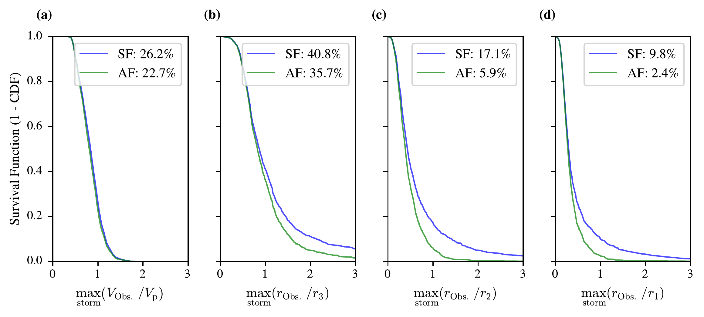
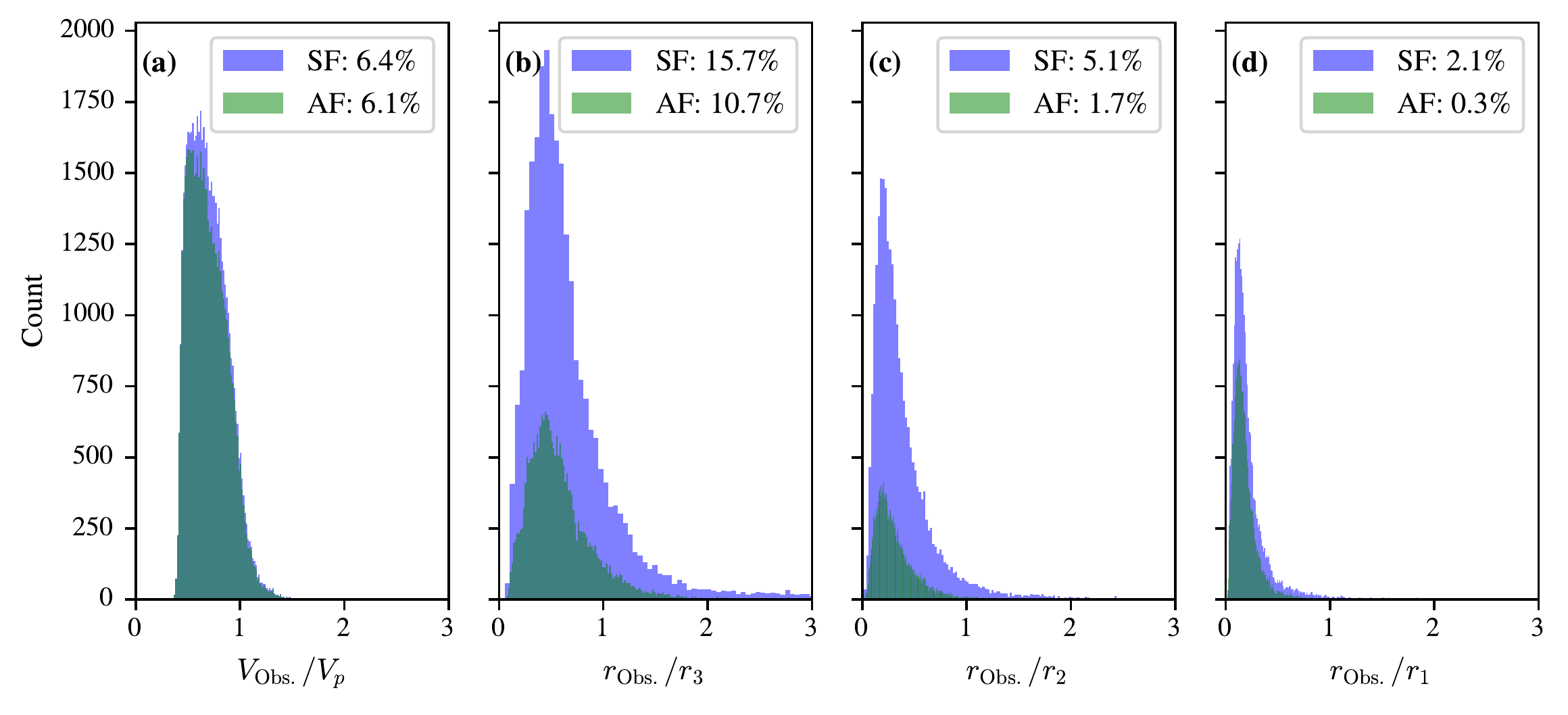
2.4.4 Superstorms: Superintense and Supersized Storms
2.4.4.0.1 Superintense storms often result from decaying potential intensity.
Table 2.8 lists the top 5 storms by maximum normalized intensity (\(V_{\mathrm{Obs.}} / V_p\)). These storms represent the most extreme cases where observed wind speeds significantly surpassed the calculated potential intensity. For some entries, the radius of maximum wind is not reported in IBTrACS, particularly outside the North Atlantic basin, precluding the calculation of normalized size. The track of the most superintense storm, Wipha (Figure 2.16) reveals a common pattern. The storms exhibit periods where \(V_{\mathrm{Obs.}}\) exceeds \(V_p\) as the potential intensity begins to rapidly decline, often due to the storm moving over colder waters or encountering unfavorable environmental conditions. For Wipha, this occurred as it approached landfall in China. This behaviour has a mechanistic explanation: \(V_p\) represents an equilibrium limit, not an instantaneous cap (Emanuel 1991). Once a TC has built up its angular momentum structure, that angular momentum cannot be rapidly destroyed by surface friction alone; the atmosphere “remembers” the storm’s prior intensity, so \(V_{\mathrm{Obs.}}\) can transiently exceed a rapidly falling \(V_p\) (Persing and Montgomery 2003). This inertial lag of TC intensity means that superintensity is especially likely during the final hours before landfall, when both the environmental PI and the storm’s internal structure are changing rapidly. An additional complication is that our monthly-mean ERA5 \(V_p\) may not capture sharp SST gradients near coastlines accurately, so the true instantaneous PI during landfall approach may differ from what ERA5 suggests. For this reason Emanuel (2000) filters storms to remove those with decaying potential intensity, although this is not implemented here.
| Time (UTC) | Name | Basin | Lon. [E] | Lat. [N] | \(\frac{V_{\text{Obs.}} }{V_{ \mathrm{p} }}\) | \(\frac{r_{\text{Obs.}}}{ r_{2}}\) | \(V_{ \mathrm{Obs.} }\)[] | \(r_{ \mathrm{Obs.} }\) [] |
|---|---|---|---|---|---|---|---|---|
| 2007-09-18 09:00 | Wipha | WP | 122.00 | 25.90 | 1.82 | 0.96 | 64.31 | 24.08 |
| 2015-03-14 18:00 | Pam | SP | 172.70 | -27.00 | 1.72 | 1.53 | 59.16 | 27.78 |
| 1992-11-21 03:00 | Hunt | WP | 144.50 | 26.70 | 1.70 | – | 56.59 | – |
| 1992-11-06 15:00 | Elsie | WP | 136.30 | 26.60 | 1.69 | – | 56.59 | – |
| 2021-12-03 03:00 | Nyatoh | WP | 139.60 | 21.80 | 1.69 | 1.24 | 63.28 | 44.45 |
lllS[table-format=4.2]S[table-format=-2.2]S[table-format=1.2]S[table-format=1.2]S[table-format=2.2]S[table-format=3.2]
Time (UTC) & Name & Basin & Lon. [E] &
Lat. [N] & \(\frac{V_{\text{Obs.}} }{V_{ \mathrm{p}
}}\) & \(\frac{r_{\text{Obs.}}}{r_{2}}\)
& \(V_{ \mathrm{Obs.}
}\)[] & \(r_{
\mathrm{Obs.} }\) []
-09-24 00:00 & Fiona & NA & -60.70 & 42.30 & 1.51
& 13.11 & 51.44 & 166.68
2012-10-29 15:00 & Sandy & NA & -72.00 & 37.70 &
1.05 & 10.72 & 42.70 & 175.94
2020-10-25 09:00 & Epsilon & NA & -53.70 & 42.60 &
0.99 & 5.90 & 33.44 & 111.12
2021-10-04 21:00 & Sam & NA & -41.90 & 45.10 & 1.13
& 5.67 & 40.13 & 74.08
2018-09-27 09:00 & Leslie & NA & -42.10 & 37.00 &
0.84 & 5.62 & 33.44 & 277.80
lllS[table-format=4.2]S[table-format=-2.2]S[table-format=1.2]S[table-format=1.2]S[table-format=2.2]S[table-format=3.2]
Time (UTC) & Name & Basin & Lon. [E] &
Lat. [N] & \(\frac{V_{\text{Obs.}} }{V_{ \mathrm{p}
}}\) & \(\frac{r_{\text{Obs.}}}{r_{2}}\)
& \(V_{ \mathrm{Obs.}
}\)[] & \(r_{
\mathrm{Obs.} }\) []
-08-30 00:00 & Ele & EP & 180.10 & 12.20 & 0.71
& 3.59 & 56.59 & 444.48
2001-08-06 18:00 & Man-Yi & WP & 145.90 & 27.30 &
1.09 & 2.86 & 59.16 & 120.38
2005-09-05 12:00 & Nabi & WP & 130.30 & 29.40 & 0.91
& 1.90 & 59.16 & 83.34
2003-09-17 00:00 & Isabel & NA & -71.50 & 28.10 &
0.74 & 1.89 & 48.87 & 101.86
2002-09-04 18:00 & Sinlaku & WP & 127.40 & 26.40 &
0.72 & 1.84 & 48.87 & 120.38
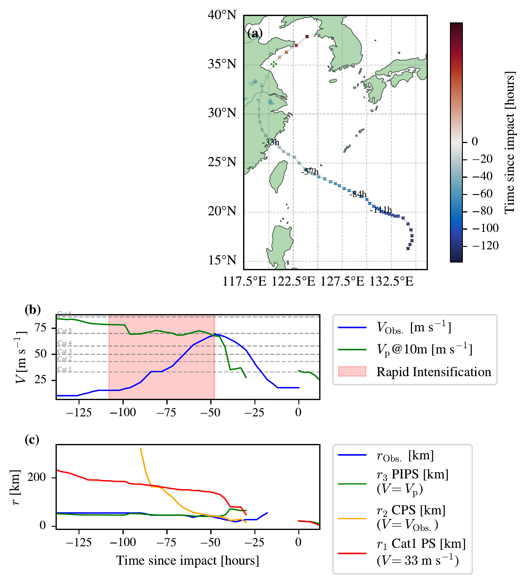
2.4.4.0.2 Supersize storms are often associated with extratropical characteristics.
Table 2.9 presents the top 5 storms by normalized corresponding potential size (\(r_{\mathrm{Obs.}} / r_2\)) before the additional filtering step. The geographical bias in RMW reporting means that North Atlantic storms are overrepresented in this table. The second most supersize storm identified is Hurricane Sandy (2012), which famously impacted the US East Coast. Sandy’s immense size has been attributed to its interaction and merger with an existing extratropical cyclone, forming a hybrid “superstorm” (Evans et al. 2017). In Figure 2.17 we can see that \(r_{\mathrm{Obs.}}\) significantly exceeded \(r_2\) after Sandy’s landfall in Cuba and remained larger throughout its northward trajectory. This case strongly suggests that the assumptions underlying purely tropical potential size derivations may not hold for storms undergoing extratropical transition or those with significant extratropical characteristics.
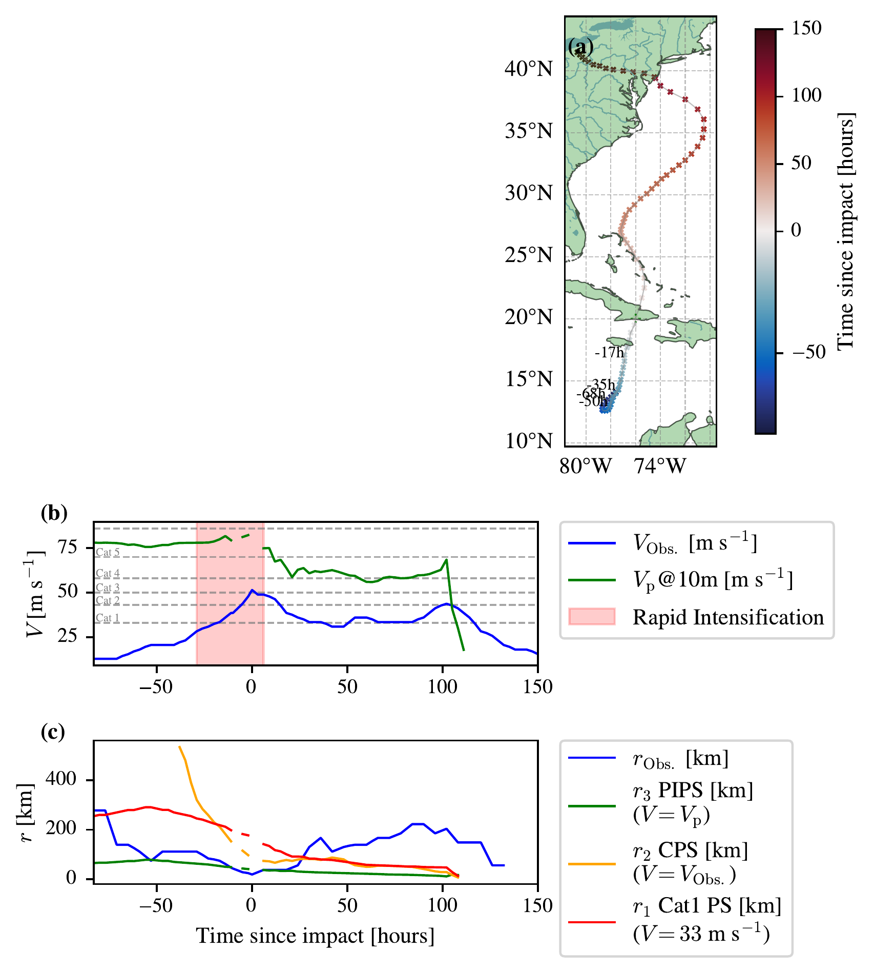
2.4.4.0.3 The remainder of supersize storms may be caused by data quality issues.
Table 2.10 shows the top 5 supersize storms after the additional filtering (AF) step (\(T_s\)\(>26.5~\degreeCelsius\), max latitude \(<\) 30 ). The new storm with the highest normalized size is Hurricane Ele (2002, EP) with max \(r_{\mathrm{Obs.}} / r_2 = 3.59\), and the second highest being Typhoon Man-Yi (2001, WP) with max \(r_{\mathrm{Obs.}} / r_2 = 2.86\). In AF, Sandy and Fiona both do not make the top 10 for supersize. Figure 2.18(a) shows the track for Hurricane Ele, which forms 10 south of Hawaii at a low latitude of 10N, travelling West before turning North-West around 300 hours before the recorded landfall. In Figure 2.18(b) we see it undergoes two periods of rapid intensification before reaching category 4 windspeed, also around 280 hours before landfall. In Figure 2.18(c) the observed radius of maximum winds, \(r_{\text{Obs.}}\), is not available for the whole track, but starts off at a very large size above 400km, then at around 270 hours before landfall it suddenly drops to less than 40km, so more than an order of magnitude. While it was recorded at its initial enormous extent, it was much larger than all of the potential sizes, but after this sudden recorded drop it is much smaller. We suggest the most likely explanation is that the hurricane in this remote location did not have enough observations to constrain its radius of maximum winds, and so it merely appears to be supersized due to poor data quality. It may be possible in the future to filter such data quality issues from the tracks before processing. Based on plotting the other supersize storms (Appendix Section Section 2.11.3), we suggest that data quality issues are probably the cause of the majority of the remaining supersize storms.
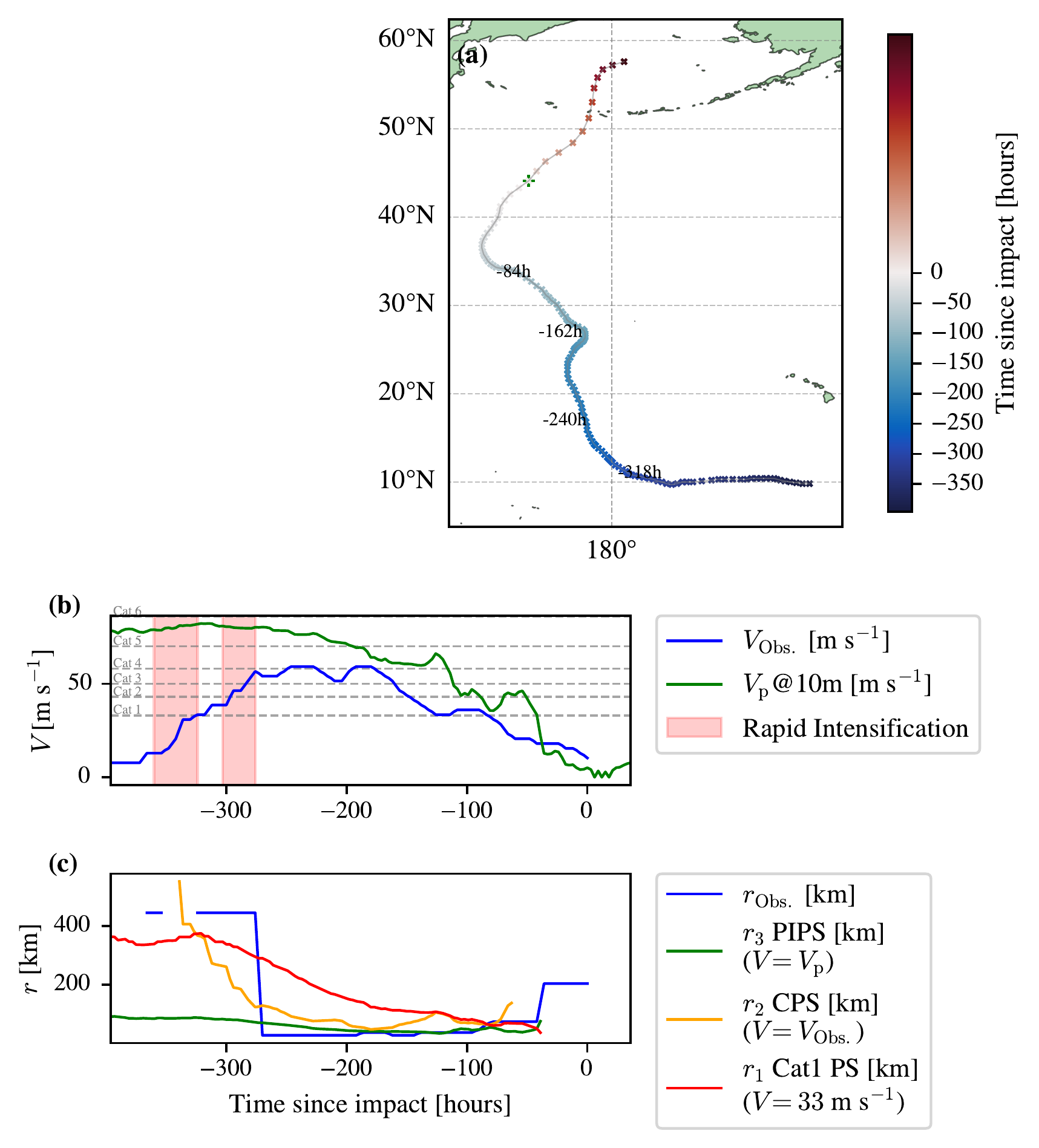
2.5 Results: Trends in Potential Intensity and Potential Sizes
2.5.1 Trends in Potential Intensity and Potential Sizes in ERA5
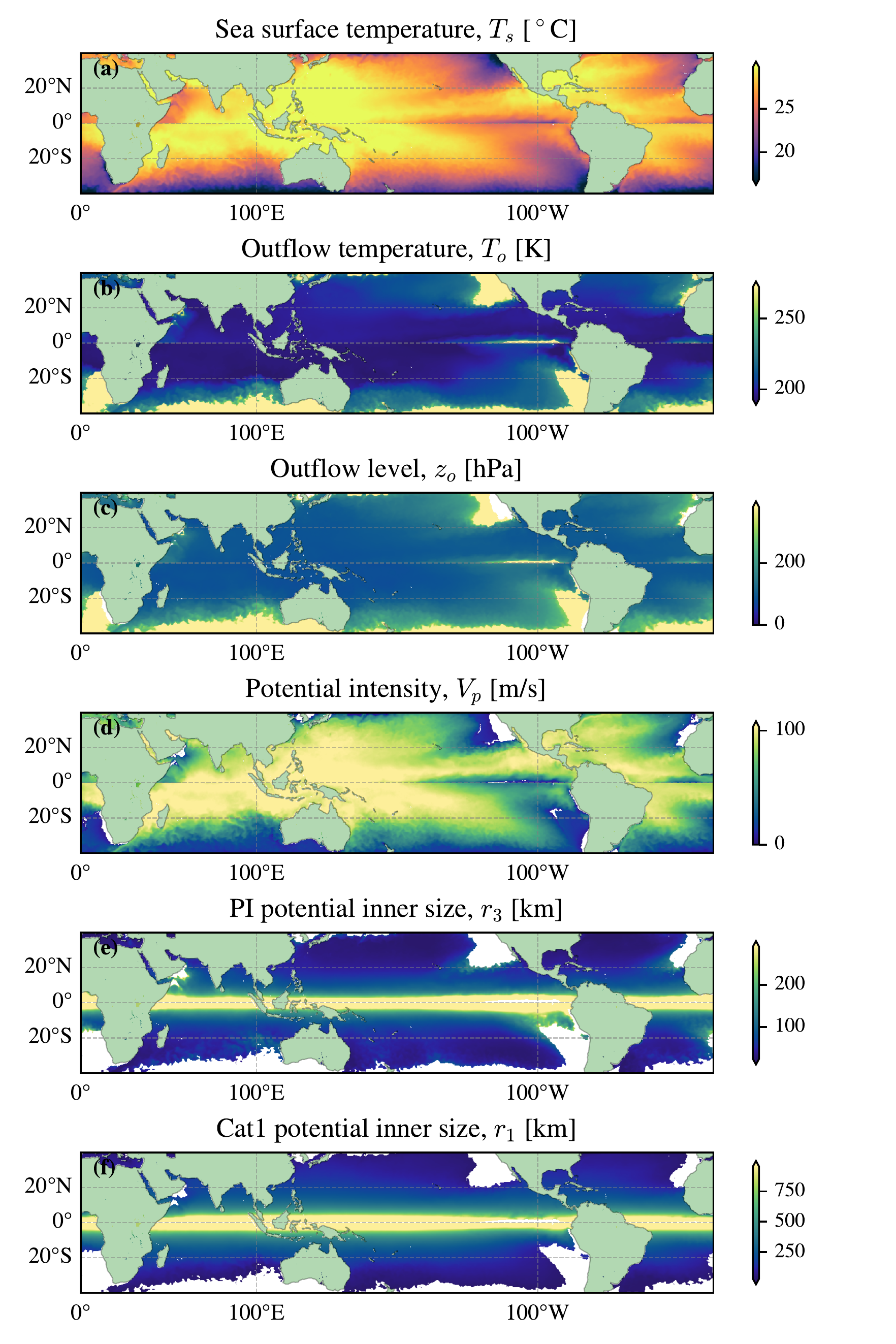
Investigating long-term trends in potential intensity and size provides crucial insights into how the environment’s capacity to support tropical cyclones is changing. First, we present global maps of sea surface temperature (\(T_s\)), potential intensity (\(V_p\)), and potential inner sizes (\(r_3\) and \(r_1\)) for August 2020 (Northern Hemisphere, NH) and February 2020 (Southern Hemisphere, SH) from the ERA5 reanalysis dataset (Figure 2.19). These maps reveal the expected patterns, with higher \(V_p\) values in the tropics and subtropics, and the potential inner sizes largely influenced by the reciprocal Coriolis parameter, \(f\), leading to larger sizes at lower latitudes. The outflow temperature, \(T_o\), and outflow pressure level, \(z_o\), have sharp edges corresponding to regions where the CAPE calculation from TCPyPI (Gilford 2021) falls back to the surface for the outflow of the moist adiabat, corresponding with the potential intensity dropping to 0 (the yellow areas in Figure 2.19(b) and the blue (zero) and white (NaN) patches in Figure 2.19(d)). These sharp edges highlight colder regions of the ocean, and in some cases are in similar positions to well-known ocean currents/fronts, such as the Agulhas return current off South Africa, which divide warmer tropical waters from colder extratropical waters. These ocean circulation effects are propagated into the potential intensities and potential size effects, so that regions associated with the cold east Pacific coastal upwelling and currents off North and South America have much lower potential intensity and potential sizes than regions at similar latitudes in the Atlantic and West Pacific.
Figure 2.20 illustrates the trends in potential intensity, \(V_p\), PI potential inner size, \(r_3\), and Cat1 potential inner size, \(r_1\), for a specific location near New Orleans over the satellite era (1980 to 2024), derived from monthly August ERA5 data. The trends are calculated using linear regression, with statistical significance assessed using the Heteroskedasticity and Autocorrelation Consistent (HAC) covariance matrix estimator (Newey and West 1987; Andrews 1991; White 1980). For this location, sea surface temperature (\(T_s\)) and potential intensity (\(V_p\)) show statistically significant increases, while the pressure level of the outflow decreases, indicating a higher outflow level over time. Although the outflow temperature (\(T_o\)) does not significantly change, this is likely due to the offsetting effects of increasing outflow level (due to warming) and the associated temperature profile. The PS potential inner size, \(r_3\), shows no significant trend, while the Category 1 potential inner size, \(r_1\), exhibits a significant increase. This could be explained by the fact that the extra energy available for the W22 sub-Carnot engine from the increase in the sea surface temperature, \(T_s\), is offset by the increase in the potential intensity, \(V_p\), so the storm cannot grow larger even though its central pressure deficit can drop.
In other words, the potential size model describes a trade-off (see Figure 2.2) between a storm’s maximum windspeed and its largest possible size (Chavas et al. 2015). The physical mechanism is angular momentum balance: the outer circulation supplies a roughly fixed angular-momentum flux to the eyewall; a more intense storm (higher \(V_p\)) must concentrate that momentum into a tighter core, so \(r_{\mathrm{max}}\) shrinks as wind speed rises, whereas a weaker storm at the same environmental conditions can spread the same momentum over a larger area and thus have a bigger \(r_{\mathrm{max}}\). According to this relationship, a less intense storm can grow larger. Climate change can alter this trade-off, allowing a larger size at the same windspeed. However, if the storm’s windspeed also increases, due to an increase in potential intensity, these two effects can offset, resulting in the same potential size.
Extending this analysis globally (Figure 2.21), we observe that potential intensity \(V_p\) generally increases across most ocean basins, consistent with global warming trends (Kossin et al. 2020). However, many areas, particularly in the East Pacific and East North Atlantic, do not show statistically significant trends, often correlating with regions where sea surface temperature increases are also not significant. Interestingly, some off-equator East Pacific regions exhibit substantial increases in outflow temperature (\(T_o\)), which can modulate the overall PI trend. The global trends for the potential sizes, \(r_3\), and \(r_1\), are shown in Figure 2.21(e)&(f) respectively. There is generally no significant trend in the PI potential inner size, \(r_3\), over the satellite era in ERA5. There is a significant increase in the Cat1 potential inner size, \(r_1\), in almost all areas, particularly in the Equator, presumably as it starts off higher (as in Figure 2.19).
One region with unexplained behaviour in Figure 2.21 is the South-Eastern tropical Pacific below the East Pacific cold tongue. In common with the cold tongue, the region has no significant trend in sea surface temperature over the satellite era (a behaviour not replicated in CMIP3/5/6 models, see e.g. Seager et al. 2019, 2022). The outflow temperature, \(T_o\), significantly increases and the outflow pressure significantly increases (corresponding to the outflow height decreasing). The region shows no trend in potential intensity \(V_p\), but the centre of this region show a large increase in PI potential inner size \(r_3\), and no trend in \(r_1\).
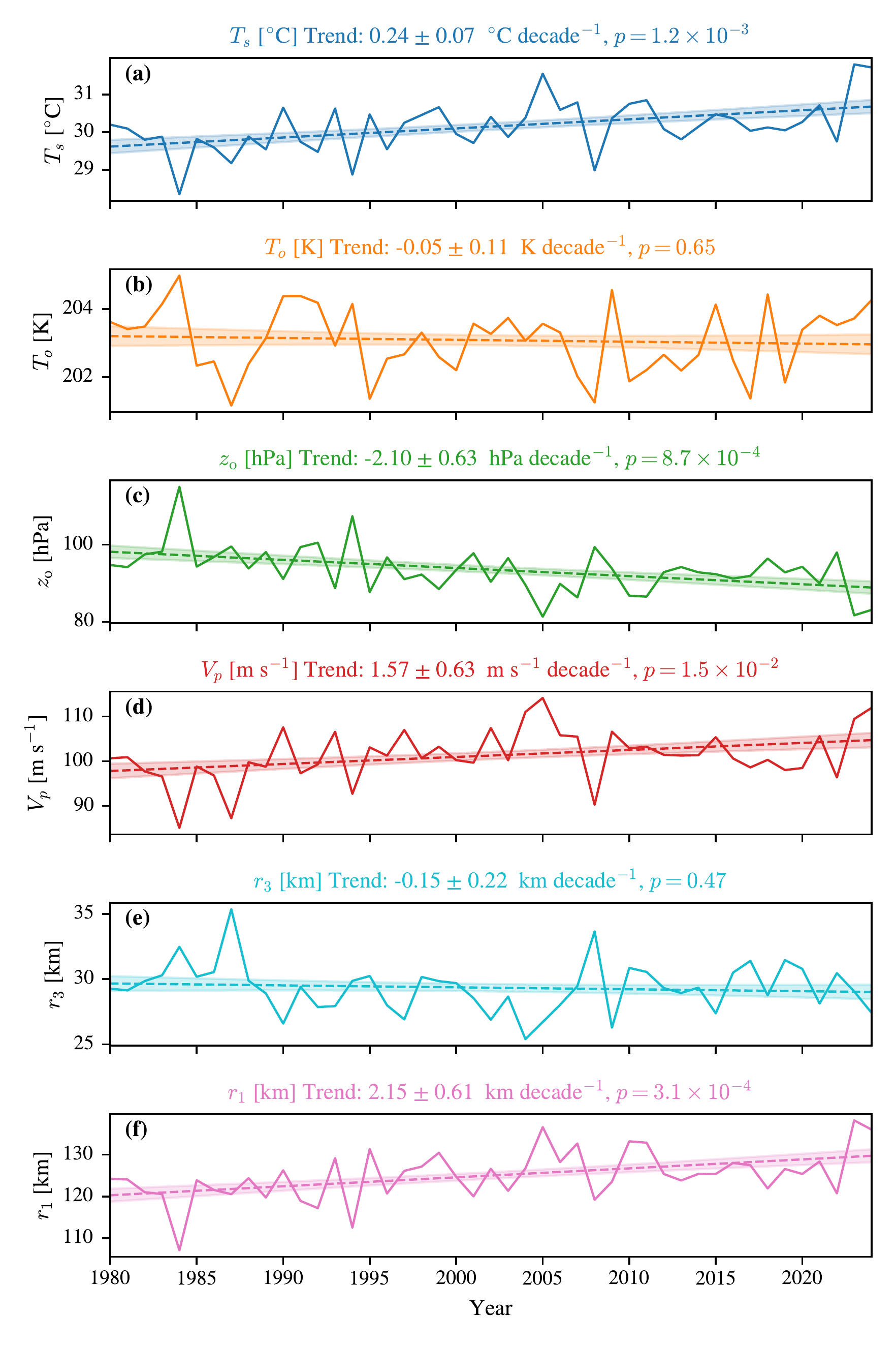
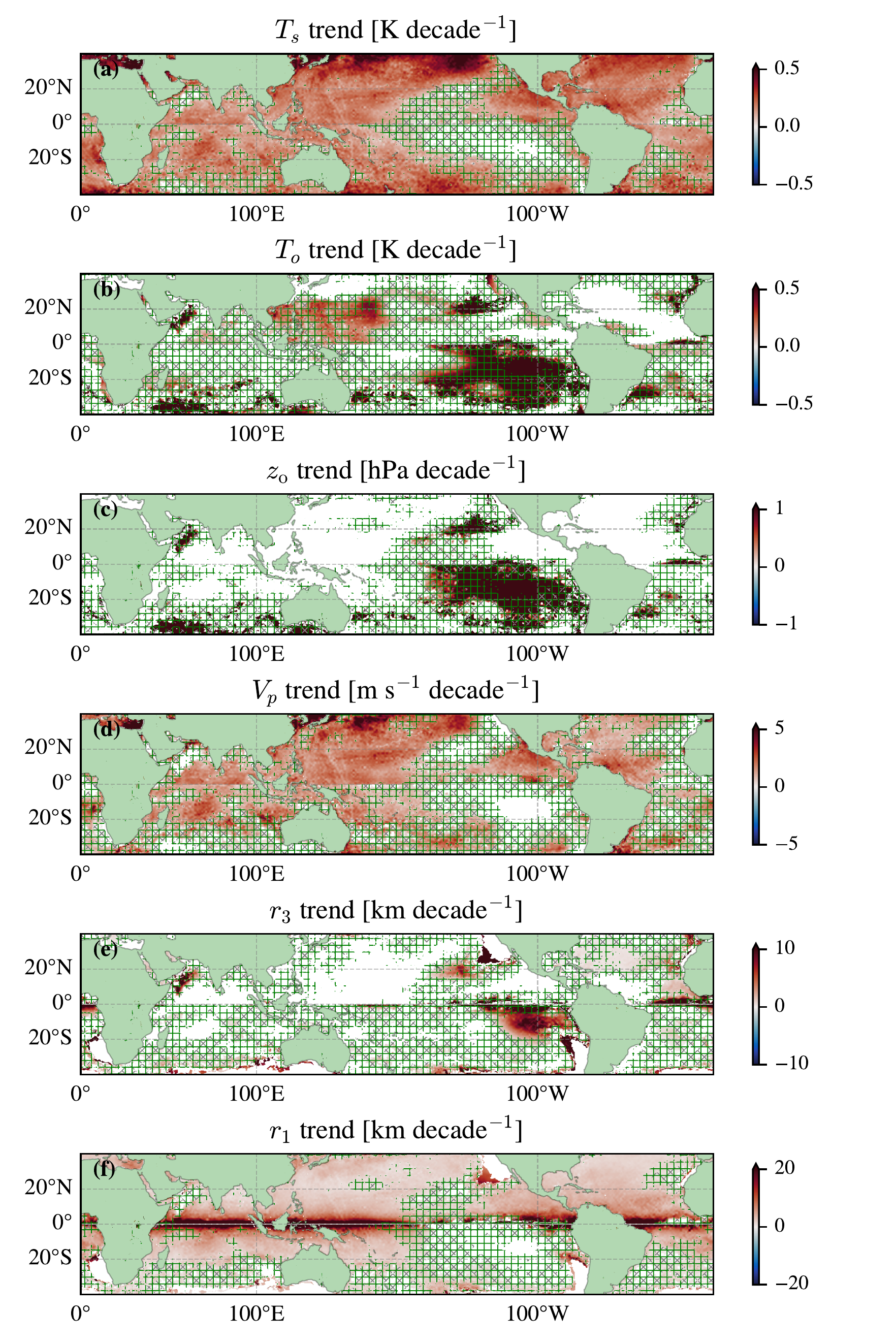
2.5.2 CMIP6 Potential Intensity and Size Projections and Bias against ERA5
As the calculation of potential size metrics is still very expensive, we limit ourselves to three CMIP6 models (CESM2, HadGEM3-GC31-MM, and MIROC6) and three ensemble members from each model. We further just consider two regions of high tropical cyclone risks: near New Orleans in the Gulf of Mexico and near Hong Kong in the South China Sea. We use data from the most extreme future scenario, SSP5-8.5, to illustrate the projected changes in \(V_p\), \(r_3\), and \(r_1\) through the 21st century.
Figure 2.22 and Figure 2.23 present projections of potential intensity and potential sizes from the three CMIP6 models (CESM2, HadGEM3-GC31-MM, and MIROC6) under the SSP5-8.5 scenario for locations near New Orleans and Hong Kong, respectively. Each figure includes a spatial panel showing the state of the variables in August 2015 (from HadGEM3-GC31-MM r1i1p1f3) and a time series panel illustrating their evolution from 1850 to 2100. The historical period (1850–2014) is derived from the models’ historical simulations, while the future period (2015–2100) follows the SSP5-8.5 scenario. We compare these projections against ERA5 reanalysis data for the historical period (1980–2024) to assess model performance, using the methods detailed in Appendix Section Section 2.10. We note an important caveat regarding the ensemble design: with only three members per model, the within-model spread (thin lines in each figure) provides a poor estimate of internal climate variability, while the spread between models reflects structural uncertainty arising from different model formulations. For projection purposes, the inter-model structural uncertainty is typically the dominant source (Hawkins and Sutton 2009); we acknowledge this limitation and present ensemble-mean trends rather than attempting a formal separation of internal and structural uncertainty.
The CESM2 model is excluded from the Hong Kong analysis due to its poor performance in simulating potential intensity in that region, as indicated by a significant positive bias when compared to ERA5 (not shown). This bias was likely as a consequence of some combination of our preprocessing step to fill in missing data at the bottom of the atmosphere, and our non-conservative bilinear regridding method using CDO (Schulzweida 2023). The HadGEM3-GC31-MM and MIROC6 models show a much smaller bias against ERA5 in this region, making them more suitable for projection analysis. HadGEM3-GC31-MM is chosen for the spatial panel in both figures as the regridded data retains features such as the Gulf Stream and Kuroshio currents clearly in the potential intensity field (see Figure 2.22 and Figure 2.23 panels (a)).
In general, the climate models show increase in almost all plotted variables over the SSP-585 scenario, including potential intensity, \(V_p\), and the potential inner sizes, \(r_3\), and \(r_1\), as well as the PI potential outer size, \(r_{a3}\). This is summarised in Table 2.11, which shows the trends in each variable for both locations and all three models. The trends are calculated using the Newey-West technique to account for autocorrelation in the data (Newey and West 1987; Andrews 1991; White 1980) on the ensemble mean. All trends are statistically significant (\(p \ll 0.05\)), apart from potential intensity \(V_p\) for the location near Hong Kong in HadGEM3-GC31-MM which is in brackets (\(p=0.7\)). For Hong Kong MIROC6 does have a positive trend in potential intensity, \(V_p\) unlike HadGEM3-GC31-MM, however in each case HadGEM3-GC31-MM has around twice the trend in each potential size metric compared to MIROC6 (56 km per decade vs 29 km per decade for \(r_{a3}\), 1.9 km per decade vs 0.79 km per decade for \(r_3\), and 6.1 km per decade vs 3.2 km per decade for \(r_1\)). For New Orleans the trends in potential intensity, \(V_p\), are similar between the three models (0.47 to 0.84 m s\(^{-1}\) per decade), and the trends in potential size metrics are also similar (23 to 27 km per decade for \(r_{a3}\), 0.31 to 0.54 km per decade for \(r_3\), and 2.6 to 2.9 km per decade for \(r_1\)). The trends in potential size metrics are much larger than those found in ERA5 over the satellite era (1980–2024) in Figure 2.21, which is unsurprising given the much stronger forcing in the SSP5-8.5 scenario compared to historical observations.
| Model | \(V_p\) [m s\(^{-1}\) dec\(^{-1}\)] | \(r_{a3}\) [km dec\(^{-1}\)] | \(r_3\) [km dec\(^{-1}\)] | \(r_1\) [km dec\(^{-1}\)] |
|---|---|---|---|---|
| Point near New Orleans | ||||
| CESM2 | 0.47 | 25 | 0.50 | 2.7 |
| HadGEM3-GC31-MM | 0.51 | 27 | 0.54 | 2.9 |
| MIROC6 | 0.84 | 23 | 0.31 | 2.6 |
| Point near Hong Kong | ||||
| HadGEM3-GC31-MM | (-0.062) | 56 | 1.9 | 6.1 |
| MIROC6 | 0.20 | 29 | 0.79 | 3.2 |
The largest interannual variability for both ERA5 and the CMIP6 models is in potential intensity (\(V_p\)), shown in Figure 2.22(b) and Figure 2.23(b), with coefficients of variation (CoV) of 5% to 7% depending on the model.15 There is much smaller interannual variability in PI potential outer size, \(r_{a3}\), (1% to 3%) and Category 1 potential inner size, \(r_1\), (CoV from 2% to 5%) as shown in Figure 2.22(d) and (h) and Figure 2.23(d) and (h). The PI potential inner size, \(r_3\), shows much higher interannual variability (CoV from 4% to 9%) than the corresponding outer size as shown in Figure 2.22(c) and Figure 2.23(c).
For the location near New Orleans, in Figure 2.22(b) there is no significant mean bias in potential intensity, \(V_p\), for the either HadGEM3-GC31-MM or CESM2 models against ERA5, although there is a positive bias in MIROC6 of \(+6.8\pm1.2\) m s\(^{-1}\).16 The PI potential outer size, \(r_{a3}\), is biased low in HadGEM3-GC31-MM (\(-116\pm 11\)km), but both CESM2 and MIROC6 have little bias against ERA5 (\(-1\pm8\) km and \(-29\pm 9\) km respectively, see Figure 2.22(d)). The PI potential inner size, \(r_3\), matches ERA5 the closest in CESM2 (a bias of \(0.0\pm0.4\) km), with MIROC6 and HadGEM3-GC31-MM both being biased low (both with \(-3.1\pm0.5\) km, see Figure 2.22(f)). Finally, the Cat1 potential inner size, \(r_1\), is biased low in HadGEM3-GC31-MM (a bias of \(-10.2\pm1.2\) km), but matches ERA5 in CESM2 and MIROC6 (\(0.0\pm0.9\) km, and \(+0.1\pm1.0\) km respectively, see Figure 2.22(h)). Based on these results, CESM2 appears to be the most reliable model for potential size and intensity for this New Orleans location, justifying its use in Chapters 3 and 4.
For the location near Hong Kong, both HadGEM3-GC31-MM and MIROC6 models have a larger potential intensity, \(V_p\), over the satellite period (1980-2024) than ERA5 (\(+9.6\pm1.3\) and \(+12.4\pm1.5\) m s\(^{-1}\) respectively, around 10%), but relatively less bias in the PI potential inner size, \(r_{a3}\) (\(-78\pm7\) km and \(-65\pm6\) km respectively, around 3%, see Figure 2.23(b) and (d)). This could be caused by a compensating error that a larger potential intensity, \(V_p\), means that the storm cannot grow larger even though there is more energy available than in ERA5. The PI potential inner size, \(r_3\), is biased low in both models compared to ERA5 (\(-3.1\pm0.9\) km and \(-0.5\pm1.0\) km respectively, see Figure 2.23(f)), which highlights even though both sizes are coherent outputs of the same potential size model at the same intensity, they can have different biases and trends in climate models. Finally, the Category 1 potential inner size, \(r_1\), does not have a substantial bias against ERA5 in either model (\(-3.1\pm0.9\) km and \(-0.5\pm1.0\) km see Figure 2.23(h)).
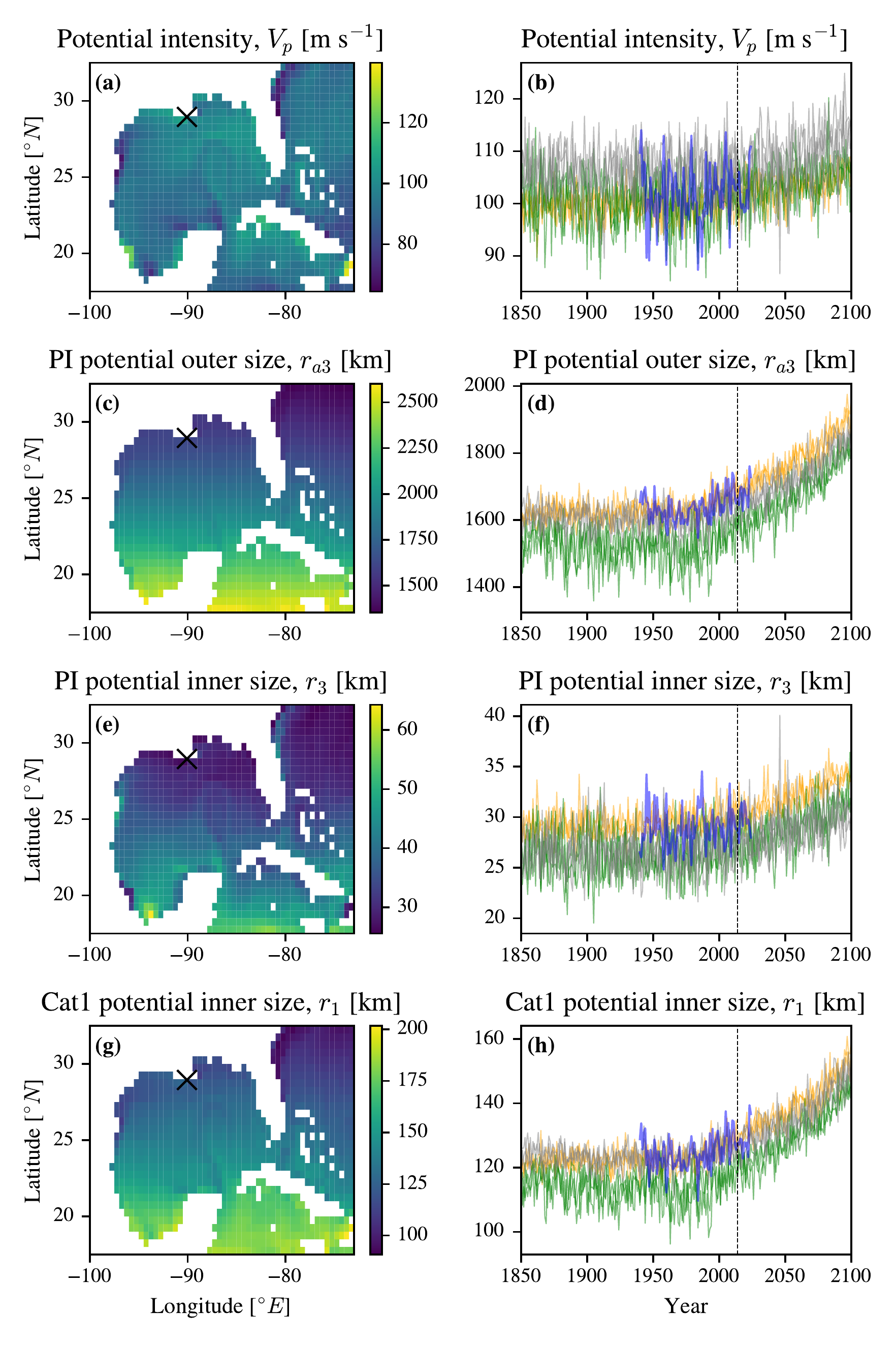
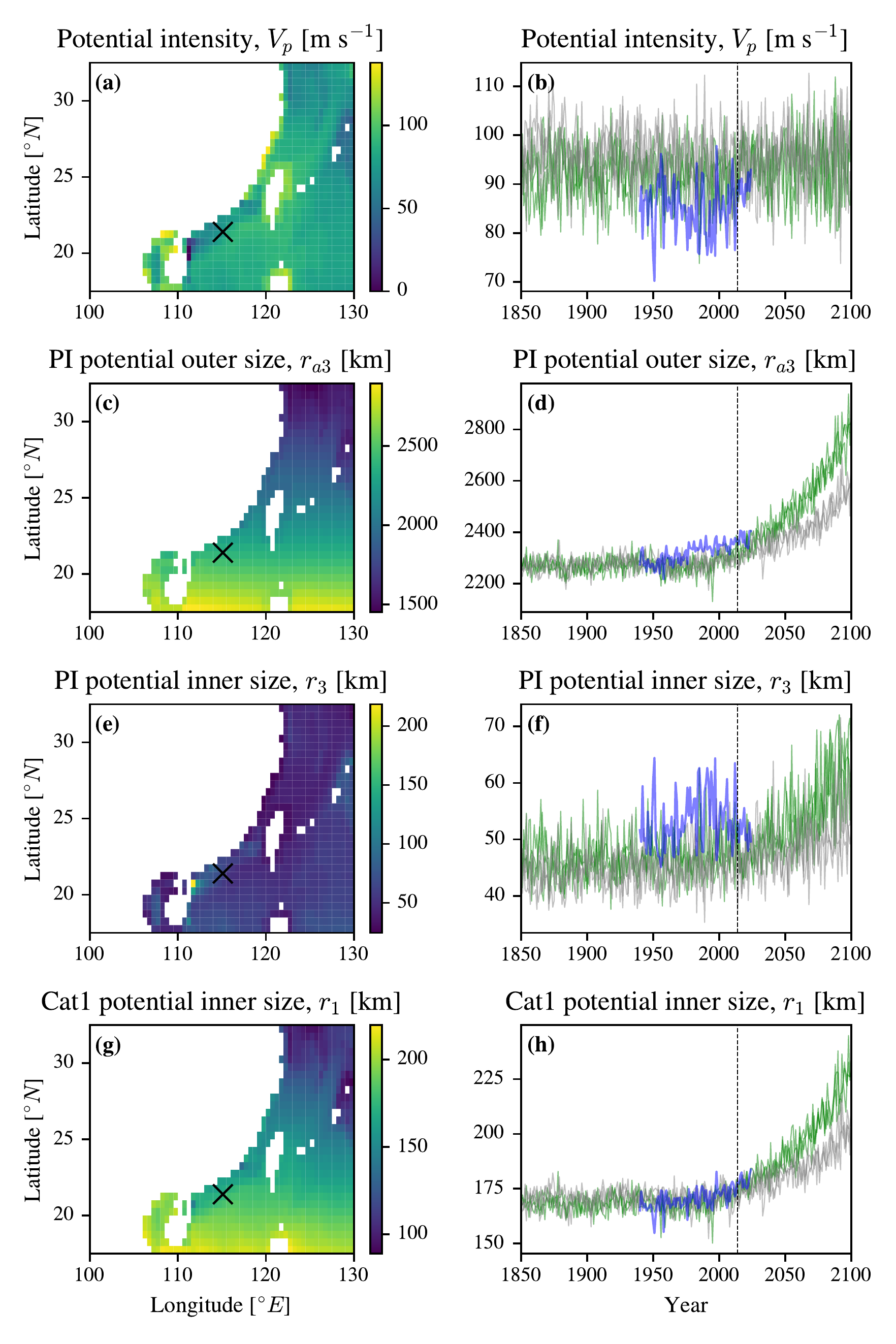
2.6 Discussion
2.6.1 Potential Size Comparison and Theoretical Consistency
Our analysis demonstrates the utility of comparing potential size and intensity metrics against observed tropical cyclone properties from the IBTrACS dataset. We consistently find that for the majority of tropical cyclones, the potential intensity, \(V_p\), is greater than the observed maximum wind speed, \(V_{\mathrm{Obs.}}\), and the various measures of potential size (\(r_3\), \(r_2\), \(r_1\)) are generally larger than the observed radius of maximum winds, \(r_{\mathrm{Obs.}}\). This aligns with the theoretical expectation that potential metrics represent upper bounds or characteristic scales that are not always reached by real-world storms due to various limiting factors (e.g., vertical wind shear, dry air intrusion, land interaction, etc.).
2.6.2 Discussion of Superintensity and Supersize
The observed phenomena of superintensity and supersize, where \(V_{\mathrm{Obs.}} / V_p > 1\) or \(r_{\mathrm{Obs.}} / r_2 > 1\), respectively, represent critical areas for further research. These exceedances challenge the completeness of current model frameworks and can arise from a combination of factors:
Observational Data Errors: Best track estimates of tropical cyclone properties, including maximum wind speed (often derived from the Dvorak technique) and radius of maximum winds, are subject to inherent uncertainties and inaccuracies (Velden et al. 2006; Knapp et al. 2018). The IBTrACS dataset, while the most comprehensive global archive, is a compilation from multiple agencies with varying methodologies, leading to inhomogeneities (Knapp et al. 2010). Even within the satellite era (1980–2024), the observing system has evolved substantially: expanding satellite coverage, the introduction and gradual expansion of aircraft reconnaissance, and successive revisions to Dvorak technique calibration all change what is recorded over time, meaning that apparent trends in \(V_{\mathrm{Obs.}}\) or \(r_{\mathrm{Obs.}}\) may partly reflect improvements in measurement capability rather than genuine physical changes in TC characteristics (Kossin et al. 2020). Our choice of the 1980–2024 period deliberately avoids the most unreliable pre-satellite records and mitigates the worst inhomogeneities, but the within-era caveat remains and should be borne in mind when interpreting any trend results. Furthermore, the record suffers from significant data gaps, with over half of all storms lacking crucial size information, and the quality of data degrades substantially in the pre-satellite era (Xu et al. 2024). These uncertainties can lead to apparent exceedances that may not be physically real, as we suggest for Hurricane Ele.
Limitations of ERA5 Monthly Data: Our use of monthly averaged ERA5 reanalysis data for calculating potential intensity and size may not fully capture sub-monthly variations in environmental conditions. ERA5 has relatively coarse spatial resolution (approx. 28 ), and monthly data further smooths the environment, potentially missing transient features like localized warm ocean eddies with high Ocean Heat Content (OHC) that can fuel rapid intensification (Goni et al. 2009), or marine heatwaves, or the storm’s self-induced cold wake, a negative feedback mechanism that is averaged out (Karnauskas et al. 2021; Zarzycki 2016) if the whole month is taken. A storm experiencing a higher instantaneous potential intensity than calculated from monthly averages could thus appear superintense or supersized even if this would not be true if we used higher temporal resolution data. We used monthly data mainly because of the currently very high computational cost of calculating potential size metrics, but future work could explore whether the same metrics calculated on hourly ERA5 data would reduce or increase the number of exceedances.
ERA5 Temporal Homogeneity: The ERA5 reanalysis assimilates an observing network that has expanded from approximately 0.75 × 10⁶ observations per day in 1979 to approximately 24 × 106 per day by 2018 (Hersbach et al. 2020), raising questions about the temporal homogeneity of derived fields such as potential intensity and size over the satellite era. For temperature at pressure levels relevant to potential intensity calculations (surface to approximately 100 ), Kozubek et al. (2020) found that ERA5 is largely free of significant temporal discontinuities, with fewer inhomogeneities than other modern reanalyses such as MERRA-2; discontinuities become apparent only well into the stratosphere (above 10 ). At the tropical tropopause, which sets the outflow temperature used in potential intensity theory, Tegtmeier et al. (2020) showed that ERA5 has the smallest warm bias of any current reanalysis (approximately 0.05 at the cold-point tropopause), benefiting from 21 model levels in the tropical tropopause layer, the highest vertical resolution among the reanalyses they evaluated. The transitions from TOVS to ATOVS satellite instruments around 1998–1999, and the assimilation of COSMIC GPS radio-occultation data from 2006 onward, produced step-like improvements in ERA5 temperature agreement with radiosonde observations at these levels (Tegtmeier et al. 2020). For moisture, Simmons (2022) identified a shift in ERA5 total-column water vapour over tropical oceans between 1987 and 1991, attributed to the introduction of SSM/I microwave-imager data into the assimilation; moisture trends from ERA5 are more temporally consistent after 1991. More broadly, Simmons (2022) demonstrated that ERA5 background-forecast trends closely match the corresponding analysis trends throughout the troposphere, indicating that the derived trends are not an artefact of the changing observing system. We note that sea surface temperatures in ERA5 are prescribed from independent observational analyses (Hersbach et al. 2020) and are not generated by the atmospheric data assimilation, so their temporal consistency, which directly affects potential intensity through both the surface enthalpy flux and the thermodynamic efficiency, is governed by the quality of the underlying SST products.
Assumptions in Potential Model Derivations: The model derivations of potential intensity and size rely on specific assumptions that can be violated in real-world storms.
Superintensity and Gradient Wind Imbalance: The PI theory tacitly assumes the storm’s boundary layer is in gradient wind balance. In reality, surface friction drives persistent inward flow below the gradient wind balance level; as this flow converges into the eyewall it can overshoot the balanced state, producing a supergradient jet: winds that locally exceed the gradient-wind value by roughly 5–20% (Kepert and Wang 2001; Smith et al. 2009). In intense storms this supergradient excess can be substantial, allowing the near-surface wind speed to breach the PI limit derived under the assumption of perfectly balanced flow (Rousseau-Rizzi and Emanuel 2019; Persing and Montgomery 2003). Superintensity is therefore a manifestation of these unbalanced boundary-layer dynamics, which are not captured by the standard PI formulation (Makarieva and Nefiodov 2023, 2025).
Supersize and Extratropical Transition: The potential size models assume a purely tropical, warm-core system. This assumption breaks down during extratropical transition (ET), when a TC interacts with mid-latitude systems and transforms into a cold-core, baroclinic cyclone (Cheung et al. 2025). This process often involves a dramatic expansion of the wind field, leading to observed sizes far exceeding those predicted by tropical potential size models (Nguyen and Schenkel 2025; Ribberink et al. 2025). The supersize storms identified in our analysis, such as Hurricane Sandy, are classic examples of storms undergoing ET or hybridization (Davis 2012; Galarneau et al. 2013; Blake et al. 2013). We were able to test this hypothesis by comparing the dataset with additional filtering (AF) to the original dataset with standard filtering (SF), and we show that when this is applied the problem of the supersize storms is greatly reduced, with the percentage of storms ever becoming supersized decreasing from 17.1% to 5.9%, and the most extreme supersize ratio decreasing from 13.1 to 3.6 (which itself is likely a observational data quality issue, see Section Section 2.4.4.0.3). Whilst the AF filters make the potential size model agree with observations, they conversely strongly suggest that the potential size model could be a misleading upper bound for storms at latitudes \(>30~\degree\) or sea surface temperatures \(<26.5~\degreeCelsius\) where ET is possible.
Wind Profile Model Assumptions: The potential size calculations rely on the CLE15 wind profile model, which itself assumes an infinitesimal transition between the convective inner core and the quiescent outer region (Chavas et al. 2015). This simplification neglects the role of intermittent convection in spiral rainbands at intermediate radii, leading to a systematic underestimation of winds in this transition zone (Chavas et al. 2015).
The intersection of these factors likely contributes to the observed exceedances. For instance, a storm undergoing rapid intensification in a localized warm ocean eddy (not fully captured by monthly ERA5) might appear superintense due to both environmental misrepresentation and observational uncertainty.
2.6.3 Parameter Choices
We use a standard reduction factor of, \(V_{\text{reduc}} \approx 0.8\), to convert tropical cyclone gradient-level winds to 10m winds over open water or vice-versa (Powell et al. 2003; Powell and Uhlhorn 2008). However, this constant factor neglects dynamically important asymmetries driven by storm motion (Kepert 2001), variations due to TC size and intensity (Giammanco et al. 2013) and the critical impact of varying surface roughness during landfall, which require more complex boundary layer models (Vickery et al. 2000; Powell 1982).
The potential size model includes several key parameter choices that could influence the results, and we only investigate the default values from D. Wang et al. (2022) (\(\beta_l=\frac{5}{4},\; \gamma_{sg}=1.2,\; \eta=0.5,\; r_o \to \infty\), \(w_{\mathrm{cool}}=0.002 \text{m s}^{-1}\)). These parameters could have been selected by D. Wang et al. (2022) both based on existing TC understanding and to best fit their high resolution \(f\)-plane simulations for tropical cyclones. D. Wang et al. (2022) do explore the sensitivity of the TC potential size to these parameters, but we should certainly explore how they affect the ability of potential inner size to match observations in future work. D. Wang et al. (2022)’s corrigendum, Wang et al. (2023), highlights that the value of \(w_{\mathrm{cool}}\) has a small effect on their potential size results, which should reduce concerns about this parameter choice.
2.6.4 Theoretical Consistency of Potential Intensity and Size Models
There is a tension in the definition of PI potential inner size, \(r_3\). On the one hand, we assume the storm is at its potential intensity, \(V_p\), a speed that was derived assuming a perfect and simplified Carnot engine running between the sea surface and the outflow with perfect gradient flow. We then use this intensity as the maximum velocity constraint for the potential size model that assumes the storm really is a much more complex sub-Carnot engine with supergradient winds and running between the near surface air temperature (assumed 1K colder than the SST) and the same outflow. Even though using potential intensity was suggested in D. Wang et al. (2022), this inconsistency is thermodynamically incongruent. However, as both models seem to work in practice, with very intense storms approaching this \(r_3\) limit for e.g. Katrina before landfall. At the moment the potential size model is a trade-off between radius and intensity, with no obvious boundary to pick for the intensity. Indeed, given that there is no velocity scale specified in the potential size model, we may as well choose the potential intensity in order to be consistent with the rest of the literature unless we can think of another way of deriving a upper bound to intensity. The resulting CLE15 profile is a completely consistent output of the potential size model, even if the choice of intensity could be improved. There are a variety of alternatives to Bister and Emanuel (2002) potential intensity that could be used instead, each making their own assumptions that could be more consistent with the potential size model.
2.6.5 Trends, Projections, and Model Biases
For potential intensity, \(V_p\), and TC intensity more broadly, there is a clear consensus that climate change will likely lead to an increase in the overall intensity of TCs (Knutson et al. 2020). Our results for ERA5 reanalysis align with this consensus, with significant trends over the satellite era in potential intensity in most areas shown. While one CMIP6 model does not project an increase in potential intensity near Hong Kong, this is more likely due to a problem with our data processing pipeline, rather than a genuine projection of no increase in potential intensity in this region. The rest of our CMIP6 results show significant increases in potential intensity, \(V_p\), consistent with the broader literature, and the thermodynamic effects of a warming climate in e.g. the Gulf of Mexico (Kossin et al. 2020).
In contrast there is no consensus on whether TC size either is changing or will change in the future (Knutson et al. 2020). Observations of tropical cyclone size are very limited, and so the record is often insufficient to calculate any significant trends. Despite these issues, Shi et al. (2024) found a global increase in the area of the TC ocean surface wave footprint of 6% per decade from 1979-2022 from ERA5 wave reanalysis, which is a proxy for an increase in TC size over this period. More broadly, lower resolution CMIP type models tend to predict larger TCs into the future (e.g. Yamada et al. 2017), which can be justified based on the increased thermodynamic fuel highlighted by the potential size model. Knutson et al. (2015) dynamically downscaled CMIP5 data and found no significant change in size over the moderate RCP4.5 climate change scenario. High resolution simulations (e.g. 2km resolution) of TCs with conditions changed to future climate scenarios tend to show a large increase in TC intensity (e.g. Kanada et al. 2013; Tsuboki et al. 2015), they project no increase in TC size. In fact, for Kanada et al. (2013) the TC intensity increases more than expected from the potential intensity increase, but the radius of maximum winds decreases rather than increasing.
We show that for ERA5 there is a significant increase in the Category 1 potential inner size, \(r_1\), in almost all areas, particularly in the equator, presumably as it starts off higher (Figure 2.19). However, there is generally no significant trend in the PI potential inner size, \(r_3\), over the satellite era in ERA5. This could be explained by the fact that the extra energy available for the W22 sub-Carnot engine from the increase in sea surface temperature, \(T_s\), is offset by the increase in potential intensity, \(V_p\), so the storm cannot grow larger even though its central pressure deficit is able to drop in response to the greater available energy in the warmer climate. In other words, the trade-off curve for potential size, \(r\left(V\right)\), (Figure 2.2) might shift up vertically in response to climate change, but if the most intense storms increase enough the net result for their PI potential size could be negligible or negative. This mirrors the effect that Kanada et al. (2013) observed in their study. This suggests the possible utility of TC potential size model as a trade-off between size and intensity for explaining existing inconsistent results in the literature. We should be able to test the hypothesis that the reason TC size is either not increasing or decreasing is because of the domination of increasing intensity, and how closely this matches the potential size model.
We also project potential size for CMIP6, where both potential inner sizes, \(r_3\) and \(r_1\), show significant increases at points near New Orleans and near Hong Kong. This is inconsistent with our ERA5 results, where \(r_1\) did not increase, could be due to a change in how the relevant input variables are changing compared to ERA5. One hypothesis from the potential size model would be that in this case the potential size tradeoff curve is rising fast enough in \(r\) that \(V_p\) is no longer rising fast enough to compensate for this change as it was in the ERA5 satellite period, and therefore the increased available energy from global warming goes to increasing the size rather than intensity of the storm. However, it could also be caused by model biases and/or the selection of the two points chosen here. Future work could investigate the precise mechanism that causes this change. This work nevertheless highlights that the potential size model could be used with CMIP6 data, and add another means to investigate how TC size could change in the future, which is, as stated, still an important unresolved question (Knutson et al. 2020).
2.6.6 The \(\beta\)-effect and Vortex Rhines Scale
All parts of the potential size and intensity model assume an \(f\)-plane, and this excludes one of the most important alternative hypotheses for explaining the limits to TC size: the vortex Rhines scale that arises from the \(\beta\)-effect (Lu and Chavas 2022; Chavas and Reed 2019). Lu and Chavas (2022) define the Rhines scale as \[\begin{equation} \text{Rh} = \sqrt{\frac{U_c}{2\pi\beta}}, \end{equation}\](2.74) where \(\beta=\frac{df}{d\varphi}\) is the variation of the coriolis parameter, \(f\), with latitude \(\varphi\), and \(U_c\) is the characteristic windspeed. In the original Rhines (1975) paper, \(U_c\) is the root-mean-square eddy velocity, a single constant characterising the energy-containing eddies of the turbulent field. For tropical cyclones, however, Lu and Chavas (2022) make a different and radius-dependent choice: they set \(U_c\) equal to the local tangential wind speed \(v(r)\), which varies across the TC vortex. This allows them to define a vortex Rhines scale that is itself a function of radius (explained further below), rather than a single fixed length scale. As \(f\sim\sin{\varphi}\) then \(\beta\sim\cos{\varphi}\), and if we assume that \(U_c\) has a weak latitudinal gradient, then \(\text{Rh}\sim \sqrt{\frac{1}{\cos{\varphi}}}\). Potential size was shown by D. Wang et al. (2022) to scale with \(|\frac{1}{f}|\sim |\frac{1}{\sin{\varphi}}|\), and so will have a singularity around the equator and decrease with increased latitude, whereas the Rhines scale, \(\text{Rh}\), will have a finite value at the equator and then increase from that value with increased latitude. The Rhines scale broadly indicates the scales beyond which Rossby wave radiation becomes more important than advection, and therefore a limit to the growth of a disturbance at that characteristic speed at that latitude (Lu and Chavas 2022).
Lu and Chavas (2022) deal with the radius-dependence of \(U_c = v(r)\) by defining the vortex Rhines scale as the radius \(r^*\) in the tropical cyclone where the Rhines scale evaluated at the local wind speed equals the radius itself, i.e. \(\mathrm{Rh}(v(r^*)) = r^*\). This self-consistent definition divides each TC into a central vortex-dominated region from an outer Rossby-wave-dominated region. Their barotropic \(\beta\)-plane simulation is initialized by the axisymmetric CLE15 profile (Chavas et al. 2015). Lu and Chavas (2022) show that storms with larger sizes compared to their vortex Rhines scale tend to shrink, and TCs equilibrate to sizes near their vortex Rhines scale.
If the Rhines scale, \(\text{Rh}\), were the dominant limit on TC size, then we would expect any increase in TC size with climate change to be caused by an increase in the characteristic windspeed, \(U_c\). If this were to scale roughly with potential intensity, \(V_p\), then the Rhines scale would increase with the square root of potential intensity, \(\text{Rh}\sim\sqrt{V_p}\). If we assume as in Section Section 2.2.1.5 that \(V_p\sim\sqrt{\Delta q}\) and that \(\Delta q\) increases roughly 7% per degree Celsius increase in sea surface temperature, \(T_s\),17 this would lead to a scaling of \(\text{Rh}\sim\sqrt[4]{T_s}\). This would be a relatively modest (and perhaps hard to detect) 1.7% per K \(T_s\) increase in TC size with global warming.
In summary, it is likely that these \(\beta\)-effect related limits become progressively more important closer to the equator, as the \(1/f\) scaling of the potential size model proposes unrealistically large TCs, that are actually limited by \(1/\beta\). If our filtering to remove extratropical transitioning storms suggests an upper latitude of around 30\(^{\circ}\) for the relevance of the potential size model, then the Rhines scale could suggest a lower latitude limit, perhaps of around 10\(^{\circ}\) above which the potential size model may be valid. In future it might be possible to combine the two models together, to give a more complete picture of the limits to TC size across the tropics.
2.6.7 Future Work and Implications
This study introduces and evaluates novel formulations of the TC potential size model, building upon the framework proposed by D. Wang et al. (2022), with a focus on the observable radius of maximum winds under various intensity assumptions. These metrics offer a valuable complement to the widely used potential intensity, \(V_p\), providing a more comprehensive understanding of TC characteristics.
2.6.7.1 Computational speed-ups are a prerequisite for more systematic CMIP6 analysis
The current computational cost of calculating potential size prevents
its routine application to large-scale datasets like the full CMIP6
ensemble. The main computational cost is the requirement to conduct a
very large number of iterations to solve the CLE15 profile, and this
must be repeated for each step in the bisection routine that finds the
potential size. Profiling reveals that around 99% of computational time
was spent calculating the CLE15 profile. Our Python implementation of
CLE15 was a large step forward in terms of computational efficiency
compared to the preexisting Octave/Matlab code (see Appendix Section Section 2.8). Nevertheless, the computational
cost of calculating potential size is still prohibitive: The 45
timesteps of the single month satellite-era ERA5 data between 40\(^{\circ}\)S and 40\(^{\circ}\)N took over 2000 node-hours on
ARCHER2 nodes with 128 CPUs each, consuming the equivalent of more than
256,000 CPU-hours in total (approximately 30 CPU-years). The problem is
embarrassingly parallel (each grid point is calculated independently)
and was parallelised across grid points using Dask distributed workers
on ARCHER2. As there are around 21 million grid-point timesteps in that
selection, this corresponds to around 44 CPU-seconds per potential size
calculation; this figure includes Dask scheduling and coordination
overheads in addition to the CLE15 computation itself, and is therefore
consistent with \(21\times10^{6} \times
44\,\mathrm{s} \approx 924\times10^{6}\) CPU-seconds \(\approx 257{,}000\) CPU-hours. Implementing
the CLE15 profile calculation in either lower-level languages, or using
Python just-in-time compilation (through e.g. numba Lam et al.
2015) could significantly reduce this processing time by at least
one order of magnitude, making both the CLE15 profile and the potential
size model more accessible for future researchers.
2.6.7.2 We should more thoroughly investigate CMIP6 model biases in potential size and intensity
Our current use of CMIP6 data to project changes in potential size into the future is more of a proof of concept than a fully reliable projection of future TC activity. Using CMIP6 models requires careful consideration of inherent model biases, and whether the trends are trustworthy. For example, CMIP6 models often project conflicting future sea surface temperature patterns, leading to large uncertainties in regional TC predictions (Wang et al. 2025), and this would also lead to significant biases in potential size and intensity. Given these biases, raw GCM output is often unsuitable for direct use in impact studies. Statistical bias correction techniques, such as quantile mapping, are a necessary step to adjust the model output’s statistical distribution to better match observations (Addisuu et al. 2025). We noted that in some locations the results seem surprising with our current CMIP6 processing pipeline (e.g. an unexpected non-significant negative potential intensity trend in HadGEM3 near Hong Kong). In general, when the computational constraints are eased, we should try to understand more systematically whether we can trust the physical mechanisms driving potential size and intensity changes in CMIP6 models, and which models are more suited for this task in each region of interest, and what forms of bias correction are sensible to apply. We note that the CESM2 model appears to be the most reliable for potential size and intensity near New Orleans, justifying its use in Chapters 3 and 4.
2.6.7.3 The Potential Height of Tropical Cyclone Storm Surges
In Chapters 3 and 4 (Thomas et al. 2025), we will utilize the PI potential size, \(r_3\), in conjunction with potential intensity, \(V_p\), for Bayesian optimization of worst-case tropical cyclone trajectories. Happily, all of the locations for which we estimate the potential height of tropical cyclone storm surges for are south of 30\(^{\circ}\)N and have oceanic SSTs in August above 26.5\(^{\circ}C\), so satisfy the criteria of the AF filter that we found excludes the majority of supersize storms, suggesting that the TC potential size model should work reasonably there. We use PI potential size, \(r_3\), because it means that we have fewer degrees of freedom for Bayesian optimization and do not need to re-run the potential size model. However, if we allowed the tropical cyclone’s wind speed to vary as an additional degree of freedom within the optimization loop, and then calculating the corresponding potential size for that windspeed, \(r_2\), the trade-off between size and intensity could be explicitly explored. This would enable the identification of the optimal point on the \(r(V)\) curve that yields the most impactful storm for a given set of climatic conditions for a given location, enabling a richer use of the TC potential size model.
2.6.7.4 Supersize could be used as a diagnostic for extratropical transition
We highlighted that many of the supersize storms identified in our analysis are likely undergoing extratropical transition (ET) or hybridization, leading to significant expansion of their wind fields beyond what is predicted by tropical potential size models. Future work could systematically investigate the relationship between supersize events and ET processes, potentially using the supersize ratio as a diagnostic tool for identifying storms undergoing ET. This could involve cross-referencing with established ET detection algorithms (Zarzycki et al. 2017) and analyzing the environmental conditions that favor such transitions.
This could be justified as a critical difference between tropical and extratropical cyclones is their source of energy: TCs derive their energy from the warm ocean surface that is in disequilibrium with the overlying atmosphere, whereas extratropical cyclones derive their energy from baroclinic processes associated with horizontal temperature gradients (Cheung et al. 2025). The potential size model assumes a purely tropical, warm-core system, and finds the full size that such a system could reach at that intensity given only this source of energy. When a storm is larger than this size, it suggests that the excess must be enabled by additional extratropical energy sources, consistent with ET.
2.7 Conclusion
We introduce the potential inner sizes of TCs, which are the radius
of maximum winds that TCs can reach with different assumptions about the
intensity (\(r_1, r_2, r_3\)). These
provide an interesting way of exploring the trade-off between size and
intensity for a TC. We show that the corresponding potential size, \(r_2\), where we assume the velocity is at
the observed intensity from IBTrACS compares favourably against the
observed size \(r_{\mathrm{Obs.}}\) for
most TCs in the IBTraCS dataset within the satellite era. This suggests
that it is a reasonable upper bound and, even when it is exceeded, it
might be used as a diagnostic to suggest that the storm has
extratropical characteristics. However, the presence of storms
undergoing extratropical transition and the exclusion of \(\beta\)-effects from the model suggests a
tentative domain of validity for the potential size model of \(c.~10^{\circ}\) to \(30^{\circ}\) latitude. This nevertheless
includes many important exposed cities such as New Orleans, Hong Kong,
and Dubai where the potential size model may be applicable. While \(r_1\) and \(r_3\) are less useful for comparing against
observations, they can both be used to explore how the potential size of
TCs changes with the maximum wind speed, and how this varies over time
and space. We show that calculating these metrics on ERA5 leads to
significant trends over the satellite era which include increasing
potential intensity and potential size in many places. The CMIP6 models
used have broadly the same trends over the historical period, and show
that under the SSP5-8.5 scenario we can likely expect the potential
intensity and size to substantially increase. The current consensus
suggests that while TC intensity and potential size are likely to
increase, the total global TC frequency may decrease even as the
proportion of intense storms rises (Knutson et al. 2020); the net
hazard implications therefore depend on both the characteristics of
individual storms and their frequency. These new metrics for the
potential size of the tropical cyclone form the basis for being able to
estimate the potential height of tropical cyclone storm surges in a
changing climate in the rest of this thesis (Chapters 3 and 4). While
our open-source computational repository, PotentialHeight
(Thomas 2025),
facilitates these calculations, further work is needed to enhance their
accessibility and computational efficiency, particularly for large
datasets. In particular we will focus on using \(r_3\) in conjunction with \(V_p\) to estimate the worst possible storm
surge height for a given set of climatic conditions. We have
demonstrated here the ability to calculate these metrics, and shown that
they capture interesting properties of the observed TCs. They are not
obviously inconsistent with IBTrACS observations, although more work
must be done to understand the discrepancies related to partially
extratropical “supersize” storms.
Acknowledgements
ST is supported by studentship 2413578 from the UKRI Centre for Doctoral Training in Application of Artificial Intelligence to the Study of Environmental Risks (grant no. EP/S022961/1). We acknowledge the World Climate Research Programme, which, through its Working Group on Coupled Modelling, coordinated and promoted CMIP6. We thank the climate modeling groups for producing and making available their model output, the Earth System Grid Federation (ESGF) for archiving the data and providing access, and the multiple funding agencies who support CMIP6 and ESGF.
Data Availability
The ERA5 data used in this study is available from the European Centre for Medium-Range Weather Forecasts (ECMWF) at https://www.ecmwf.int/en/forecasts/datasets/reanalysis-datasets/era5. The IBTrACS data is available from the National Centers for Environmental Information (NCEI) at https://www.ncdc.noaa.gov/ibtracs/. The CMIP6 data is available from the Pangeo catalogue at https://pangeo.io/catalogue.html.
Open Software
The code for this work is available at https://github.com/sdat2/PotentialHeight (Thomas 2025), and
builds upon the sithom utility library (Thomas
2024).
2.8 Appendix: Python Implementation of the Chavas et al. (2015) TC Wind Profile Model
2.8.1 Introduction
This appendix details the Python implementation of the TC wind profile model developed by Chavas et al. (2015), which merges the inner core solution of Emanuel and Rotunno (2011) and the outer profile of Emanuel (2004). The Python code serves as a translation of the original MATLAB library (Chavas 2022) and aims to replicate its functionality and outputs.
2.8.2 Model Overview
The Chavas et al. (2015) model generates a complete TC wind profile by smoothly merging two preceding profiles:
The Emanuel (2004) (E04) profile, which describes the outer region of the storm where radiative cooling and frictional decay are dominant. This profile is calculated by integrating inward from a large outer radius (\(r_A\)) where the wind speed approaches zero.
The Emanuel and Rotunno (2011) (ER11) profile, which describes the inner core of the storm, characterized by a balance between friction and the outward transport of angular momentum. This profile is typically defined relative to the radius of maximum wind (\(r_{\mathrm{max}}\)) and the gradient-level maximum wind speed (\(V_{gm}\)).
The merging process involves finding a point in non-dimensional angular momentum (\(M/M_0\)) versus non-dimensional radius (\(r/r_A\)) space where the inner and outer profiles are tangent. The final profile is then constructed by using the ER11 solution inside this merge radius and the E04 solution outside (Chavas et al. 2015).
2.8.3 Python Implementation Structure
The Python implementation is structured into several functions, mirroring the modular design of the original MATLAB code (Chavas 2022). The main entry point for calculating the wind profile is the ‘chavas_et_al_2015_profile’ function. This function orchestrates the calculations by calling several helper functions:
‘_e04_outerwind_r0input_nondim_mm0’: Calculates the non-dimensional E04 outer profile (\(M/M_0\) vs \(r/r_A\)) by integrating inward from \(r_A\). It incorporates the option for a variable drag coefficient (\(C_d\)) based on wind speed, following Donelan et al. (2004) (Chavas et al. 2015).
‘_er11_radprof_raw’: Calculates the raw ER11 profile based on input \(V_{gm}\) and either \(r_{\mathrm{max}}\) or \(r_A\). It uses an implicit relationship between \(r_{\mathrm{max}}\) and \(r_A\) (based on ER11 Eq. 37) to determine the other radius (Chavas et al. 2015).
‘_er11_radprof’: This function iteratively calls ‘_er11_radprof_raw’, adjusting the internal \(V_{gm}\) and input radius parameters until the resulting raw ER11 profile matches the target \(V_{gm}\) and input radius (\(r_{\mathrm{in}}\), which is either the target \(r_{\mathrm{max}}\) or \(r_A\)) (Chavas et al. 2015). This iterative process is necessary because \(V_{gm}\) and \(r_{\mathrm{max}}\) are interdependent in the ER11 solution.
‘_curve_intersect’: A helper function used during the merge process to find the intersection points between two curves defined by discrete data points.
‘_radprof_eyeadj’: Applies an empirical adjustment to the profile within the eye region (typically inside \(r_{\mathrm{max}}\)), scaling the wind speed based on a power law (\((r/r_{\mathrm{max}})^\alpha\)) if requested (Chavas et al. 2015).
The main ‘chavas_et_al_2015_profile’ function first computes the E04 profile, then iteratively searches for the correct non-dimensional radius of maximum wind (\(r_{\mathrm{max}}/r_A\)) by generating ER11 profiles and checking for tangency (via intersection) with the E04 profile in non-dimensional angular momentum space. Once the tangent point (merge point) is found, the final profile is constructed by combining the converged ER11 profile inside the merge radius and the E04 profile outside (Chavas et al. 2015).
2.8.4 Differences and Numerical Stability
While the Python implementation aims to be a faithful translation, certain numerical approaches differ from the original MATLAB code (Chavas 2022), which can impact stability, particularly with challenging input parameters.
Solving the \(r_{\mathrm{max}}\)-\(r_A\) Relation: In ‘ER11_radprof_raw.m’, the MATLAB code uses the ‘solve’ function from the symbolic math toolbox to find the root(s) of the equation relating \(r_{\mathrm{max}}\) and \(r_A\). This symbolic approach attempts to find exact or highly accurate solutions to the equation (Chavas et al. 2015). The Python implementation, in ‘_er11_radprof_raw’, uses ‘scipy.optimize.root_scalar’ with a numerical method (Brent’s method with bracketing). Numerical root-finding methods rely on iterative approximation within a specified range and can be sensitive to the function’s behavior, initial guesses, and the chosen bracket. For certain parameter combinations, the numerical solver might struggle to find the correct root or converge reliably, especially if the function is ill-behaved or has multiple roots close together within the physical constraints.
Curve Intersection Method: The MATLAB ‘curveintersect.m’ function uses ‘interp1’ followed by a custom inverse interpolation routine (‘mminvinterp’) to find points where the difference between two curves is zero. This custom function may handle non-monotonic data or specific edge cases more robustly (Chavas et al. 2015). The Python ‘_curve_intersect’ function uses ‘scipy.interpolate.interp1d’ and identifies intersections by detecting sign changes in the difference between the interpolated curves. While standard, this method’s accuracy and reliability depend heavily on the quality and resolution of the interpolated data and may be less robust when dealing with noisy or numerically unstable input profiles resulting from previous calculation steps.
ER11 Profile Convergence (Additive Adjustment): Both the MATLAB ‘ER11_radprof.m’ and the Python ‘_er11_radprof’ implementations use a simple additive correction based on the error in \(V_{gm}\) and \(r_{\mathrm{in}}\) to adjust the internal parameters iteratively (Chavas et al. 2015). While straightforward, this method can be prone to numerical instability and overshooting, especially when the errors are large. The Python code includes checks to reset negative \(V_{gm}\) or \(r_{\mathrm{in}}\) values
Merge Search and Fallbacks: The process of finding the tangent point (merge point) involves a bisection search on the \(r_{\mathrm{max}}/r_A\) ratio, checking for intersections between the E04 and ER11 non-dimensional angular momentum profiles (Chavas et al. 2015). If the underlying ER11 profile calculation (‘_er11_radprof’) fails for a given guess of \(r_{\mathrm{max}}/r_A\), or if ‘_curve_intersect’ fails to find reliable intersections, the bisection search can fail to converge on a valid merge point. The MATLAB code includes a fallback to increment \(C_h/C_d\) if the solution does not converge in the merge search loop, a specific strategy that might help in some difficult cases (Chavas et al. 2015). The Python implementation’s handling of this specific fallback during the merge search failure might differ or be less effective.
These differences in numerical solvers, interpolation, and convergence handling, even subtle ones, can accumulate and lead to divergence or incorrect results when the model is applied to input parameters that push the boundaries of its intended use or numerical stability limits, such as an exceptionally large outer radius. The failure of these core calculation steps leads to the propagation of invalid numerical values (NaNs), which can then cause errors in subsequent calculations downstream.
2.8.5 Verification against MATLAB Implementation
To verify the Python implementation against the original MATLAB code, we conducted a series of tests comparing the outputs of both implementations for a range of input parameters. The tests focused on the ability of the code to generate the same pressure at the radius of maximum wind speed \(p_m\), the radius of maximum wind speed \(r_{\mathrm{max}}\), and the central pressure \(p_c\) as we change the outer radius of the cyclone \(r_A\). As shown in Figure 2.24, the Python implementation produces smooth curves that closely match the MATLAB results, while the MATLAB implementation exhibits unphysical jumps in the output. This suggests that the Python implementation is more numerically stable and trustworthy than the original MATLAB code.
In addition, we compared the execution time of both implementations on different computers. The results, shown in Section 9, indicate that the Python implementation is significantly faster than the MATLAB implementation, especially on the Archer2 login node. This speed advantage is particularly important for large-scale simulations and analyses, where computational efficiency is crucial.
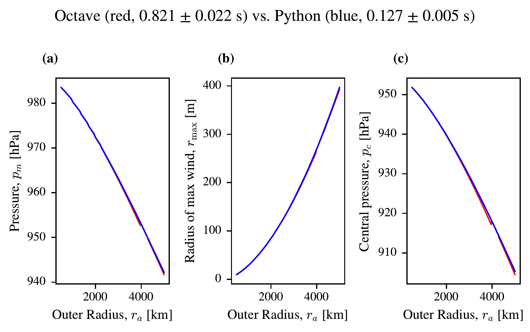
| Computer | Python Version [s] | MATLAB Version [s] |
|---|---|---|
| MacBook Pro M1 | \(0.123\pm 0.005\) | \(0.795 \pm 0.021\) |
| Archer2 Login Node | \(1.99 \pm 0.504\) | \(34.2 \pm 4.3\) |
| Archer2 Compute Node | \(0.173 \pm 0.007\) | \(1.310 \pm 0.070\) |
2.9 Appendix: Trends in Potential Size and Intensity
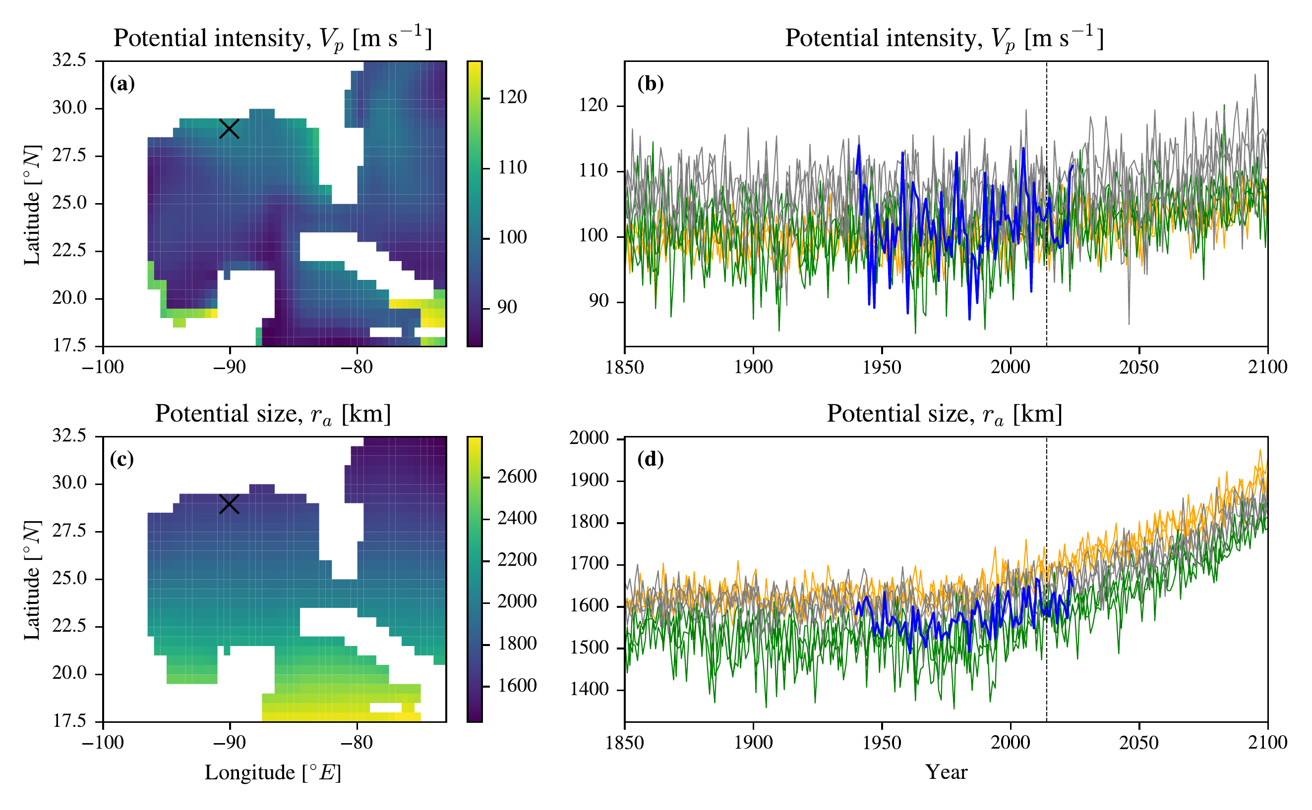
In this section, we present the results of the trends in outer radius potential size (evaluated at the potential intensity) and potential intensity for New Orleans, Louisiana, using the ERA5 reanalysis data and the CESM2 model outputs (historical from 1850-2014, ssp585 from 2014-2100). In all cases we look just at the August results. Figure 2.25 shows the spatial distribution of potential intensity and potential size over the Gulf of Mexico in August 2025 for CESM2-r4i1p1f1, as well as the time series of these variables for a point near New Orleans. The time series data is shown for three different CESM2 members (orange) and ERA5 (blue). The ERA5 data is available from 1940-2024, while the CESM2 data is available from 1850-2014 for historical runs and from 2014-2100 for SSP5-8.5.
The statistical results are summarized in Table 2.12 and Table 2.13. Table 2.12 shows the temporal correlations between potential intensity, potential size, and sea surface temperature for New Orleans. The correlations are calculated for different time periods, including the full ERA5 period (1940-2024), the recent satellite period (1980-2024) for both ERA5 and CESM2 to be able to compare results, and the SSP5-8.5 period (2014-2100) to assess future climate change implications. The correlations show that there is a strong positive correlation between potential intensity and sea surface temperature, as well as between potential size and sea surface temperature. The correlations are generally stronger in the CESM2 model outputs than in the ERA5 reanalysis.
In Figure 2.25, we see that the potential intensity, \(V_p\), and potential size, \(r_A\), show a clear trend of increasing values over time, particularly in the SSP5-8.5 scenario results up to 2100. The potential intensity, \(V_p\), appears to have a higher trend in ERA5 over the satellite period (1980-2024) than CESM2, roughly 1.3 m s\(^{-1}\) decade\(^{-1}\) compared to around 1.0 m s\(^{-1}\) for ERA5. Interestingly this is also coupled to a higher than expected apparent sensitivity to temperature of 7.3 m s\(^{-1}\) \(^\circ\)C\(^{-1}\) compared to around 4.0 m s\(^{-1}\) \(^\circ\)C\(^{-1}\) for CESM2. As PI is around 100 m s\(^{-1}\) for this point, this suggests that the PI sensitivity on \(T_s\)) is higher in ERA5 than was expected based on our analysis in Section Section 2.2.1.5. We showed that we might expect between 2.56% and 3.79% sensitivity for global temperature increase, and so approximately between 3.2% and 4.7% per \(^{\circ}\)C for \(T_s\) (given \(m=0.8\)). ERA5 appears significantly higher than this in 1980-2024, and so perhaps our assumption that the enthalpy change term scales only with the Clausius-Clapeyron relation for water vapour is too conservative in this period. This could be caused for example by changes in the relative humidity, where a decrease in relative humidity would increase the enthalpy change term and therefore \(V_p\).
However, in the SSP5-8.5 period (2014-2100) we see that the CESM2 model has a much lower sensitivity of around 1.8% per \(^{\circ}\)C for \(T_s\), or around 1.7% per \(^{\circ}\)C, which is much lower than our expected range. It also has a lower trend of 0.6 m s\(^{-1}\) decade\(^{-1}\). This suggests that PI is not increasing as fast as we might expect, suggesting that our Clausius-Clapeyron scaling is failing in a different way perhaps with increased RH, or an upper troposphere warming much faster than expected. Both of these apparent failures would be worth investigating further in future work.
For the PI potential outer size, the \(r_A\), we see a very strong trend in both ERA5 and CESM2 over the satellite period (1980-2024) of around 1.4 km yr\(^{-1}\) for ERA5 and around 1.8 km yr\(^{-1}\) for CESM2. This is coupled to a sensitivity to \(T_s\) of around 47 km \(^\circ\)C\(^{-1}\) for ERA5 and around 55 km \(^\circ\)C\(^{-1}\) for CESM2. In the SSP5-8.5 period (2014-2100), we see that the trend in \(r_A\) increases even further to around 9.0 km yr\(^{-1}\) for CESM2, coupled to a sensitivity to \(T_s\) of around 96 km \(^\circ\)C\(^{-1}\). This suggests that the potential size of TCs could increase dramatically in a warming climate, which could lead to much larger storm surges and increased risk to coastal communities. We have no expected range for the sensitivity of \(r_A\), but the problems highlighted in the \(V_p\) sensitivity suggest that we should be cautious in interpreting these results, as there could be significant data issues or model biases that are affecting the results.
| Member | Start | End | \(\rho(V_p, t)\) | \(\rho(r_A, t)\) | \(\rho(T_s, t)\) | \(\rho(T_s, V_p)\) | \(\rho(T_s, r_A)\) |
|---|---|---|---|---|---|---|---|
| ERA5 | 1940 | 2024 | 0.08 | 0.40 | 0.30 | 0.86 | 0.64 |
| ERA5 | 1980 | 2024 | 0.31 | 0.45 | 0.44 | 0.88 | 0.72 |
| CESM2-r4i1p1f1 | 1980 | 2024 | 0.45 | 0.71 | 0.85 | 0.69 | 0.81 |
| CESM2-r10i1p1f1 | 1980 | 2024 | 0.20 | 0.50 | 0.71 | 0.62 | 0.81 |
| CESM2-r11i1p1f1 | 1980 | 2024 | 0.54 | 0.66 | 0.84 | 0.75 | 0.81 |
| CESM2-r4i1p1f1 | 2014 | 2100 | 0.59 | 0.90 | 0.97 | 0.70 | 0.96 |
| CESM2-r10i1p1f1 | 2014 | 2100 | 0.45 | 0.90 | 0.96 | 0.60 | 0.95 |
| CESM2-r11i1p1f1 | 2014 | 2100 | 0.45 | 0.90 | 0.96 | 0.59 | 0.95 |
| Member | Start | End | \(m(t, V_p)\) | \(m(t, r_A)\) | \(m(T_s, r_A)\) | \(m(T_s, V_p)\) |
| [\(\text{m s}^{-1}\;\text{yr}^{-1}\)] | [\(\text{km}\;\text{yr}^{-1}\)] | [\(\text{km}\;^{\circ}\text{C}^{-1}\)] | [\(\text{m s}^{-1}\;^{\circ}\text{C}^{-1}\)] | |||
| ERA5 | 1940 | 2024 | \(\left(2 \pm 3\right)\times 10^{-2}\) | \(\left(7 \pm 2\right)\times 10^{-1}\) | \(\left(4.3 \pm 0.6\right)\times 10^{1}\) | \(7.8 \pm 0.5\) |
| ERA5 | 1980 | 2024 | \(\left(1.3 \pm 0.6\right)\times 10^{-1}\) | \(1.4 \pm 0.4\) | \(\left(4.7 \pm 0.7\right)\times 10^{1}\) | \(7.3 \pm 0.6\) |
| r4i1p1f1 | 1980 | 2024 | \(\left(1.0 \pm 0.3\right)\times 10^{-1}\) | \(1.8 \pm 0.3\) | \(\left(5.5 \pm 0.6\right)\times 10^{1}\) | \(4.0 \pm 0.6\) |
| r10i1p1f1 | 1980 | 2024 | \(\left(5 \pm 3\right)\times 10^{-2}\) | \(1.6 \pm 0.4\) | \(\left(7.1 \pm 0.8\right)\times 10^{1}\) | \(4.0 \pm 0.8\) |
| r11i1p1f1 | 1980 | 2024 | \(\left(1.2 \pm 0.3\right)\times 10^{-1}\) | \(1.9 \pm 0.3\) | \(\left(5.9 \pm 0.7\right)\times 10^{1}\) | \(4.3 \pm 0.6\) |
| r4i1p1f1 | 2014 | 2100 | \(\left(7 \pm 1\right)\times 10^{-2}\) | \(2.5 \pm 0.1\) | \(\left(6.3 \pm 0.2\right)\times 10^{1}\) | \(1.9 \pm 0.2\) |
| r10i1p1f1 | 2014 | 2100 | \(\left(6 \pm 1\right)\times 10^{-2}\) | \(2.5 \pm 0.1\) | \(\left(6.0 \pm 0.2\right)\times 10^{1}\) | \(1.8 \pm 0.3\) |
| r11i1p1f1 | 2014 | 2100 | \(\left(5 \pm 1\right)\times 10^{-2}\) | \(2.5 \pm 0.1\) | \(\left(6.2 \pm 0.2\right)\times 10^{1}\) | \(1.5 \pm 0.2\) |
2.10 Appendix: Additional CMIP6 Statistical Results
2.10.1 Coefficient of Variation Calculation
The coefficient of variation (CV) is a standardized, dimensionless measure of the dispersion of a probability distribution or frequency distribution. It is often referred to as relative variability as it quantifies the degree of variability relative to the mean of the data (Everitt and Skrondal 2010). It is defined as the ratio of the standard deviation, \(\sigma\), to the absolute value of the mean, \(\mu\), \[\begin{equation} CV = \frac{\sigma}{|\mu|}. \end{equation}\](2.75) The primary advantage of the CV is that it allows for a direct comparison of variability between datasets that may have different units. The standard CV can be misleading if the data contains a long-term trend (i.e., is non-stationary). A simple warming trend, for example, will increase the overall standard deviation of a temperature time series, but this increase is due to the secular change, not the year-to-year fluctuations.
To isolate the true interannual variability, we use a detrended coefficient of variation. This is calculated in two steps. First, a linear trend is fitted to the time series, and the residuals, the deviations of each data point from the trend line, are calculated. Second, the standard deviation of these residuals, \(\sigma_{\text{resid}}\), is computed. This value, which represents the variability around the long-term trend, is then normalized by the mean of the original, non-detrended time series, \(|\mu_{\text{orig}}|\), \[\begin{equation} CV_{\text{detrended}} = \frac{\sigma_{\text{resid}}}{|\mu_{\text{orig}}|}. \end{equation}\](2.76) This metric provides a more meaningful measure of how much a quantity fluctuates from year to year, effectively separating the stationary variability from any underlying long-term trend.
Table 2.11 shows the coefficient of variation for potential intensity and potential size for New Orleans and Hong Kong. The coefficient of variation is a measure of relative variability, calculated as the standard deviation divided by the mean. The results show that the coefficient of variation is generally low for both potential intensity and potential size, indicating that the models are relatively consistent in their predictions. However, there is some variability between models and locations, with some models showing higher coefficients of variation than others.
| Model | \(r_{a3}\) | \(r_1\) | \(r_3\) | \(V_p\) |
|---|---|---|---|---|
| Point near New Orleans | ||||
| CESM2 | \(0.02 \pm 0.00\) | \(0.03 \pm 0.00\) | \(0.08 \pm 0.00\) | \(0.05 \pm 0.00\) |
| HadGEM3-GC31-MM | \(0.01 \pm 0.00\) | \(0.02 \pm 0.00\) | \(0.08 \pm 0.01\) | \(0.06 \pm 0.00\) |
| MIROC6 | \(0.01 \pm 0.00\) | \(0.03 \pm 0.00\) | \(0.09 \pm 0.00\) | \(0.07 \pm 0.00\) |
| Point near Hong Kong | ||||
| CESM2 | \(0.02 \pm 0.00\) | \(0.02 \pm 0.01\) | \(0.04 \pm 0.00\) | \(0.03 \pm 0.00\) |
| HadGEM3-GC31-MM | \(0.03 \pm 0.01\) | \(0.05 \pm 0.01\) | \(0.08 \pm 0.00\) | \(0.05 \pm 0.00\) |
| MIROC6 | \(0.02 \pm 0.00\) | \(0.03 \pm 0.00\) | \(0.08 \pm 0.00\) | \(0.05 \pm 0.00\) |
2.10.2 Mean Bias and Bias Trend Calculation
To assess the systematic bias of each CMIP6 model against the ERA5 reanalysis, we account for the hierarchical structure of the data, where three distinct ensemble members are nested within each parent model, by employing a linear mixed-effects model (Gelman and Hill 2007). This approach is statistically necessary because the time series from different members of the same model (e.g., the three members of CESM2) are not independent; they share the same model physics and respond to the same external forcings. Simply concatenating the three time series and performing a standard regression would constitute pseudoreplication, leading to artificially small standard errors and an overestimation of statistical significance (Gelman and Hill 2007).
The mixed-effects model allows us to estimate the overall, shared bias of the model (the fixed effect) while explicitly partitioning out the variability between its members (the random effect). The model for the bias, \(y_{ij}\), (defined as CMIP6 minus ERA5) at time step, \(i\), for ensemble member, \(j\), is specified as, \[\begin{equation} y_{ij} = (\beta_0 + u_{0j}) + \beta_1 t_i + \epsilon_{ij}, \end{equation}\](2.77) where:
\(\beta_0\) is the fixed intercept, representing the average bias of the parent CMIP6 model (e.g., HadGEM3-GC31-MM) against ERA5 across the entire analysis period.
\(\beta_1\) is the fixed slope, representing the average trend in this bias over time \(t_i\). A non-zero slope indicates that the model’s bias relative to ERA5 is changing over time.
\(u_{0j}\) is the random intercept for a specific member \(j\) (e.g., ‘r1i1p1f3‘). It quantifies how much that particular member’s mean bias deviates from the overall parent model’s mean bias \(\beta_0\). These random effects are assumed to follow a normal distribution, \(u_{0j} \sim \mathcal{N}(0, \sigma_u^2)\), where the variance \(\sigma_u^2\) is a robust measure of the inter-member spread caused by internal climate variability.
\(\epsilon_{ij}\) is the residual error for a specific data point, assumed to be \(\epsilon_{ij} \sim \mathcal{N}(0, \sigma_\epsilon^2)\).
This formulation yields a single, robust estimate for each CMIP6 model’s core bias and bias trend, with uncertainties that correctly account for the data structure. It should be noted that while this method addresses the non-independence across ensemble members, it does not explicitly correct for temporal autocorrelation within each time series, which can be addressed using alternative methods like Newey-West standard errors on the ensemble-mean series.
Table 2.12 shows the results of a mixed-effects model to assess the bias in potential intensity and potential size for New Orleans and Hong Kong. The results show the mean bias and bias trend for each model at both locations, along with the standard error. The results indicate that there are significant biases in both potential intensity and potential size for all models at both locations, with some models showing larger biases than others. The bias trends also vary between models and locations, with some models showing increasing biases over time while others show decreasing biases.
| Mean Bias | ||||
|---|---|---|---|---|
| Model | \(r_{a3}\) [km] | \(r_1\) [km] | \(r_3\) [km] | \(V_p\) [m s\(^{-1}\)] |
| Point near New Orleans | ||||
| CESM2 | \(-1 \pm 8\) | \(0.0 \pm 0.9\) | \(0.0 \pm 0.4\) | \(0 \pm 1\) |
| HadGEM3-GC31-MM | \(-116 \pm 11\) | \(-10.2 \pm 1.2\) | \(-3.1 \pm 0.5\) | \(-0.2 \pm 1.1\) |
| MIROC6 | \(-29 \pm 9\) | \(0.1 \pm 1.0\) | \(-3.1 \pm 0.5\) | \(6.8 \pm 1.2\) |
| Point near Hong Kong | ||||
| CESM2 | \(-35 \pm 9\) | \(13.9 \pm 1.1\) | \(-22.5 \pm 0.9\) | \(36.3 \pm 1.4\) |
| HadGEM3-GC31-MM | \(-78 \pm 7\) | \(-3.1 \pm 0.9\) | \(-10.4 \pm 1.0\) | \(9.6 \pm 1.3\) |
| MIROC6 | \(-65 \pm 6\) | \(-0.5 \pm 1.0\) | \(-11.7 \pm 1.1\) | \(12.4 \pm 1.5\) |
| Bias Trend | ||||
| Model | \(r_{a3}\) [km yr\(^{-1}\)] | \(r_1\) [km yr\(^{-1}\)] | \(r_3\) [km yr\(^{-1}\)] | \(V_p\) [m s\(^{-1}\) yr\(^{-1}\)] |
| Point near New Orleans | ||||
| CESM2 | \(0.3 \pm 0.3\) | \(0.01 \pm 0.04\) | \(0.026 \pm 0.015\) | \(-0.05 \pm 0.04\) |
| HadGEM3-GC31-MM | \(0.4 \pm 0.4\) | \(0.02 \pm 0.05\) | \(0.027 \pm 0.018\) | \(-0.04 \pm 0.05\) |
| MIROC6 | \(0.0 \pm 0.3\) | \(-0.06 \pm 0.04\) | \(0.040 \pm 0.018\) | \(-0.11 \pm 0.05\) |
| Point near Hong Kong | ||||
| CESM2 | \(1.2 \pm 0.3\) | \(0.02 \pm 0.04\) | \(0.16 \pm 0.03\) | \(-0.13 \pm 0.06\) |
| HadGEM3-GC31-MM | \(1.0 \pm 0.3\) | \(0.03 \pm 0.04\) | \(0.16 \pm 0.04\) | \(-0.13 \pm 0.05\) |
| MIROC6 | \(0.2 \pm 0.2\) | \(-0.08 \pm 0.04\) | \(0.15 \pm 0.04\) | \(-0.17 \pm 0.06\) |
2.11 Appendix: Additional Track Examples
2.11.1 Notable TCs
Notable storms, such as Ida (2021), Harvey (2017), Ian (2022), Saola (2023), Bebinca (2018), Mangkhut (2018), and Freddy (2023), are presented in Figures Figure 2.26 through Figure 2.32. These examples highlight a range of behaviors: some storms, like Ida, show periods of rapid intensification where \(V_{\mathrm{Obs.}}\) approaches \(V_p\), while others, like Bebinca, consistently remain well below their potential intensity. The relationship between observed and potential sizes also varies, with some storms consistently smaller than their potential size (e.g., Mangkhut) and others, particularly weaker storms or those undergoing extratropical transition, exceeding \(r_3\) or even \(r_2\) (e.g., Harvey, Freddy during weak phases). Mangkhut (Figure 2.31) presents a prominent case where observed intensity exceeded potential intensity for an extended period, indicating a “superintense” event.
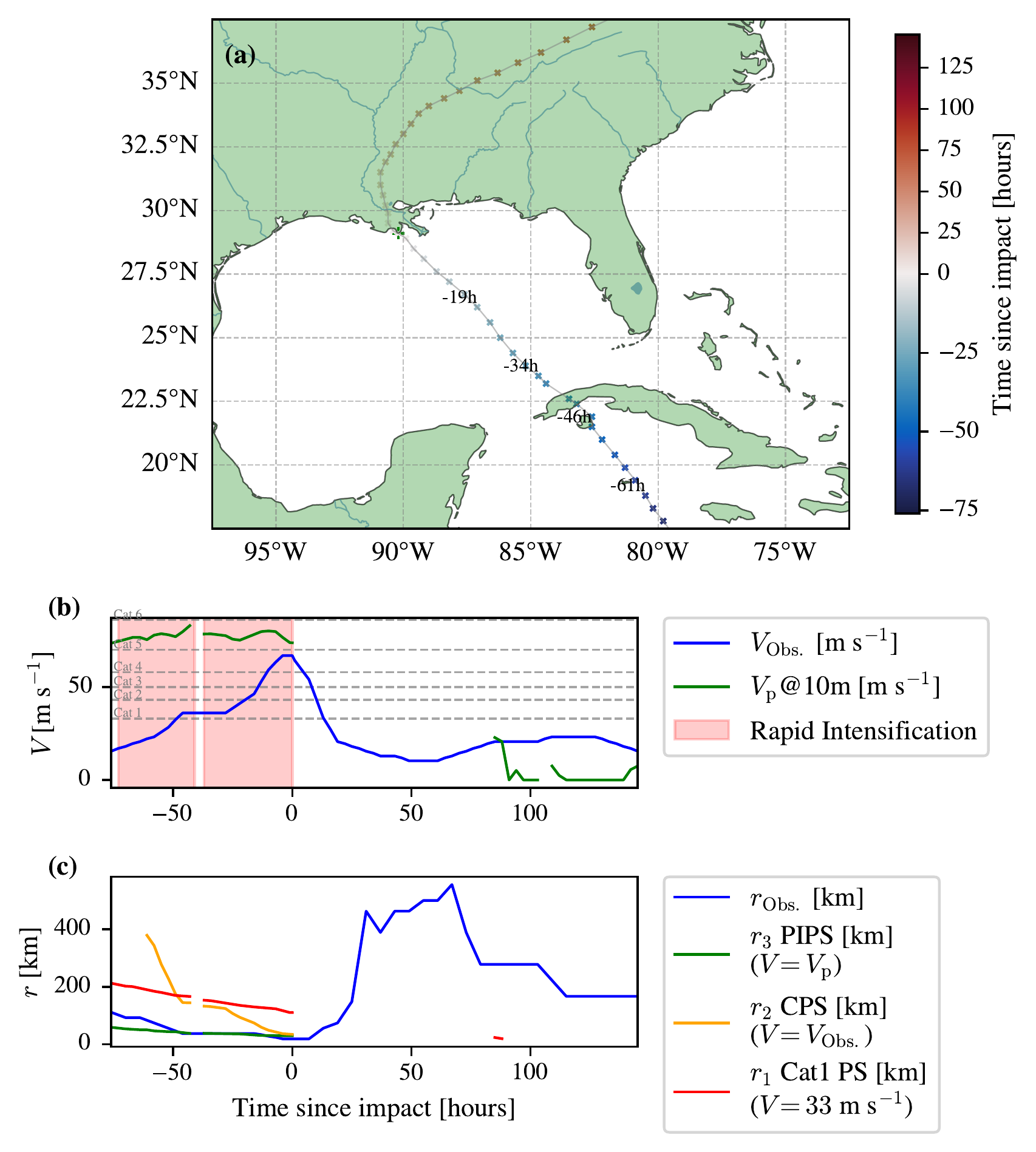
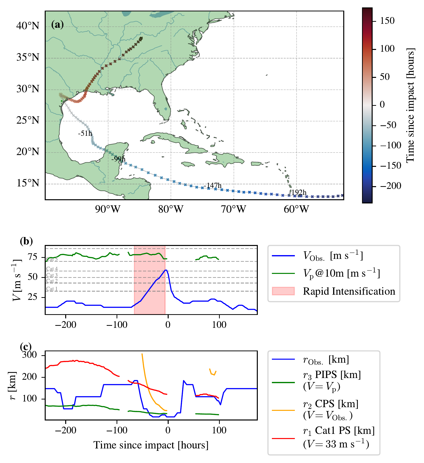
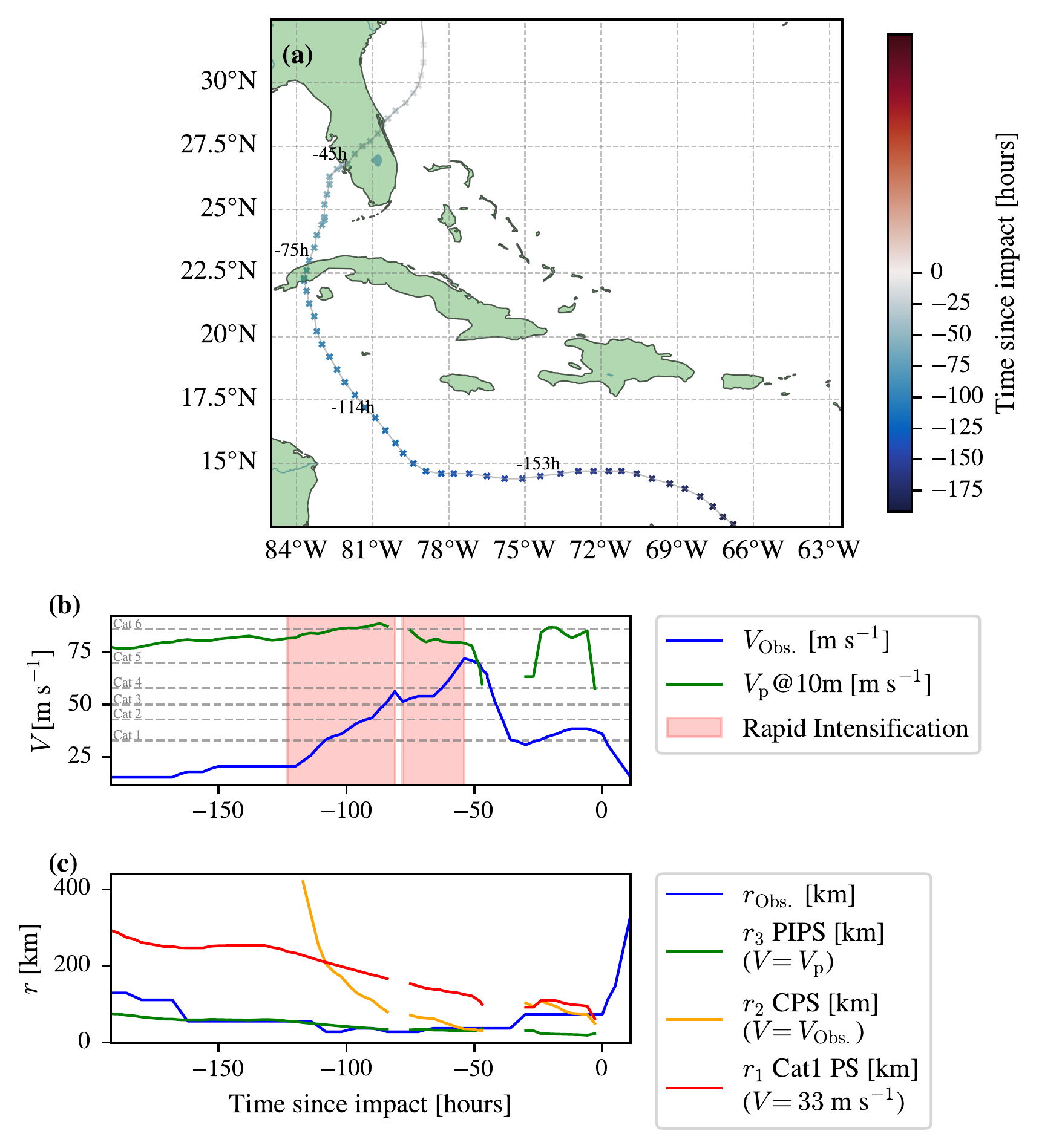
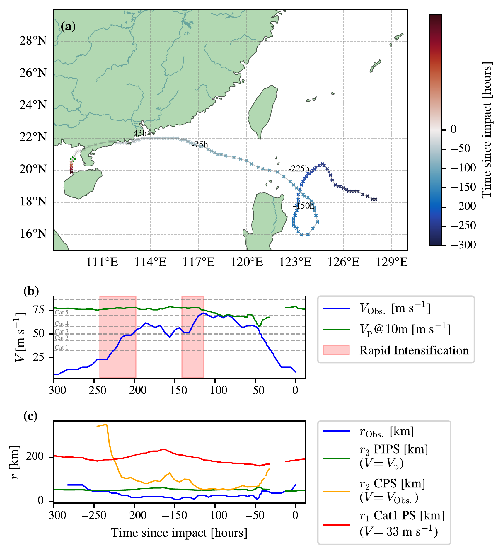
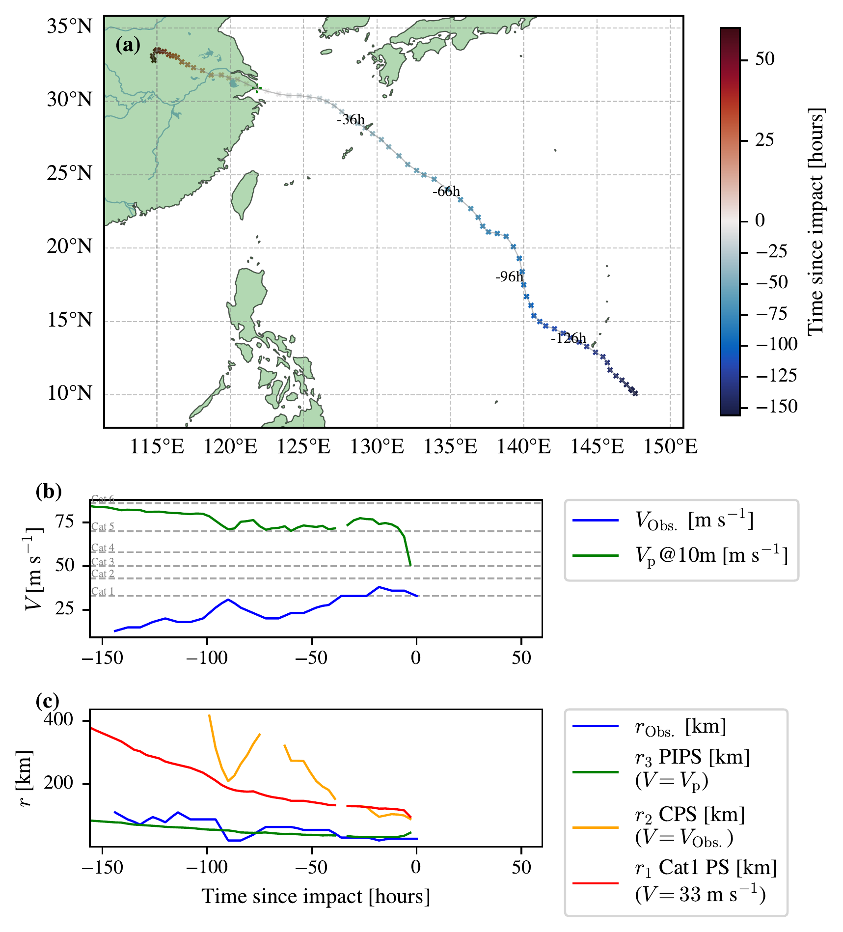
2.11.2 Superintense Example: TC Pam (2015)
Pam (2015) is the second most superintense storm in our database, with \(V_{\mathrm{Obs.}} / V_p = 1.72\). Similar to Wipha, \(V_{\mathrm{Obs.}}\) exceeds \(V_p\) as the storm moves into an environment where \(V_p\) rapidly declines, likely due to colder waters and extratropical transition. This is shown in Figure 2.33.
2.11.3 Supersize Examples
Fiona (2022) is the most supersize storm in our database with standard filtering, with \(r_{\mathrm{Obs.}} / r_2 = 13.11\). Its supersize is observed as it tracks northward, potentially undergoing extratropical transition over cooler waters or ocean fronts. This is shown in Figure 2.34.
2.12 Appendix: Additional Exceedance Rate Sensitivity Analysis
We also want to understand the sensitivity of these exceedance rates to the applied intensity thresholds without any additional filtering. This is explored in Figure 2.36 & Figure 2.35. Varying the lower limit for observed wind speed (\(V_{\mathrm{Obs.}}\)) primarily impacts the exceedance of \(r_3\), as filtering out low-intensity storms reduces the number of cases where a large observed size might contradict the assumption of \(V=V_p\) inherent in \(r_3\). Conversely, changing the lower bound of potential intensity (\(V_p\)) generally reduces the likelihood of all measures being exceeded. The most pronounced decrease is observed for \(r_3\), declining from 16 exceedance at \(V_p=33~\meter\per\second\) to 8 at \(V_p=70~\meter\per\second\). This trend suggests that in environments with higher potential intensity, where the energy source is more definitively tropical, the assumptions underlying these potential metrics may become more robust, leading to fewer exceedances.
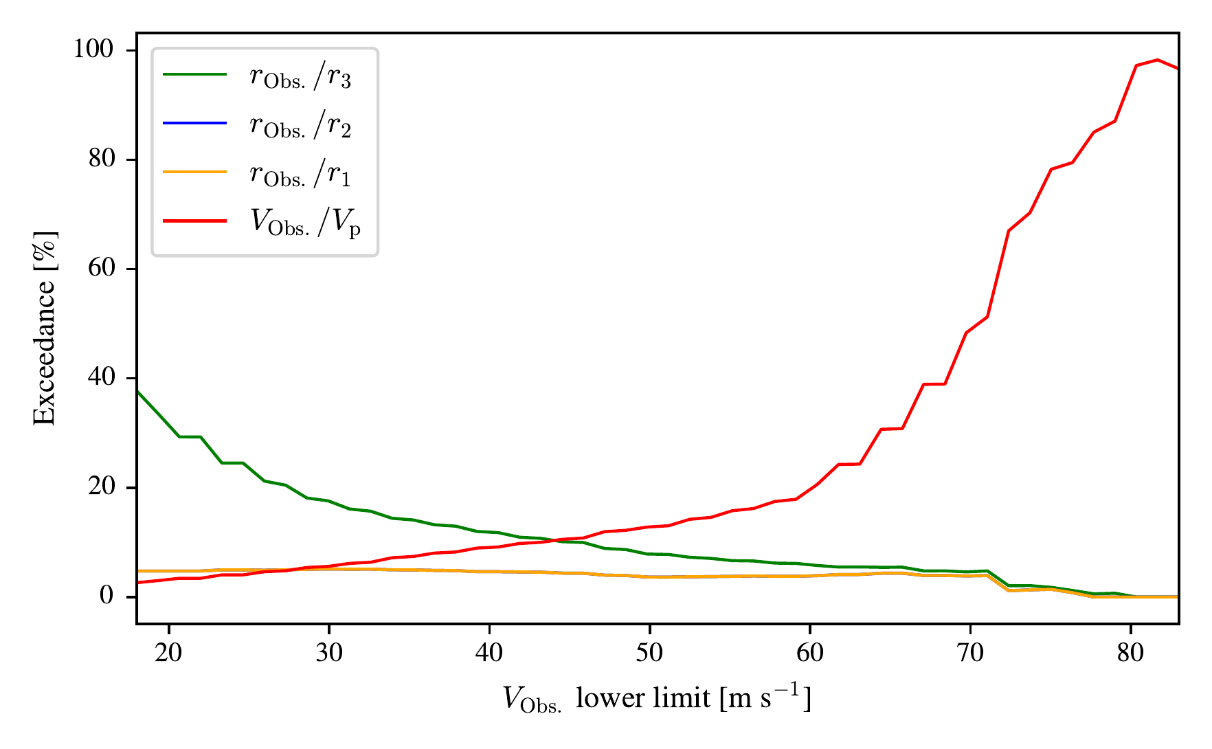
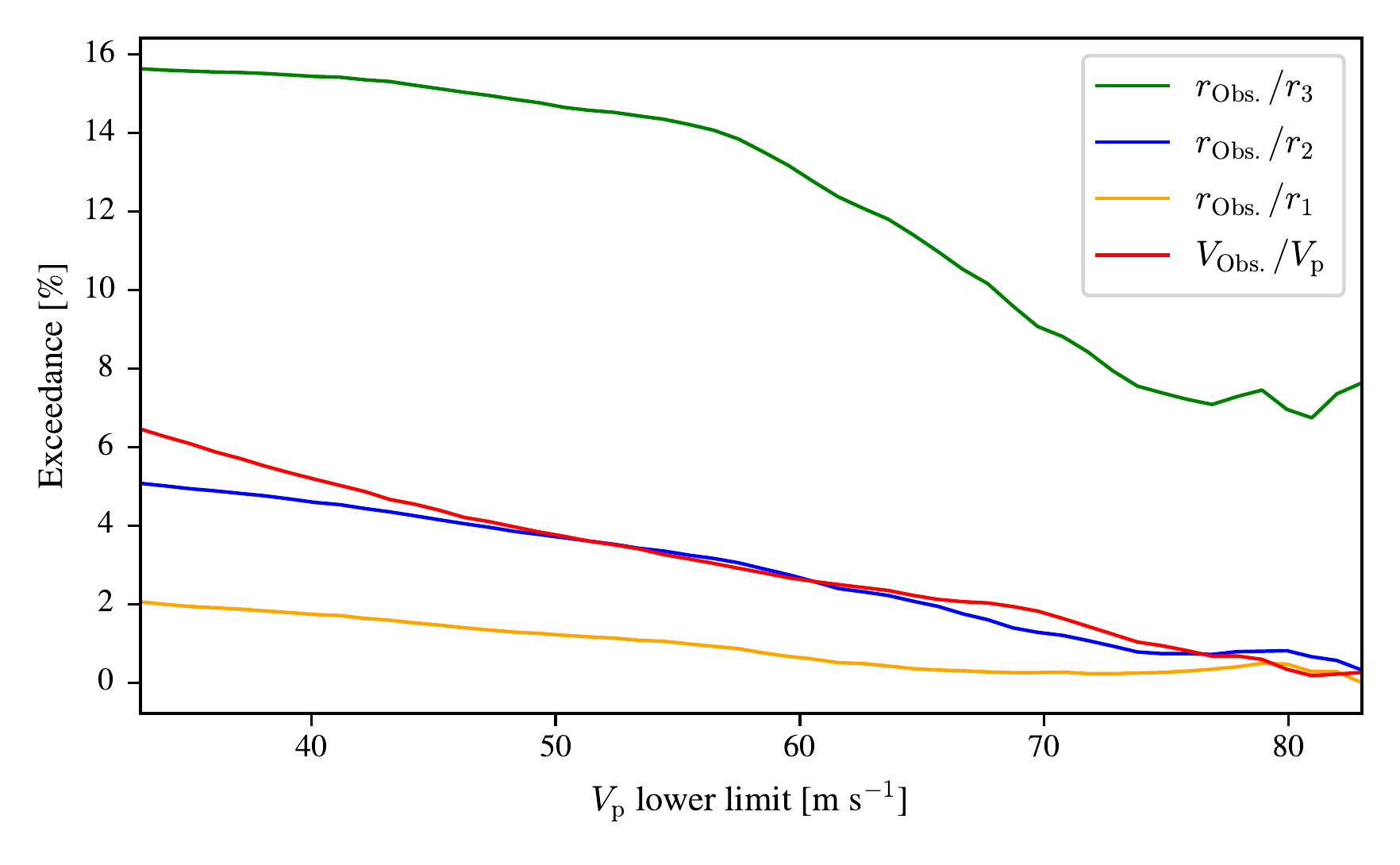
References
Typically the area between the tropics of Capricorn and Cancer, both at \(23.4^{\circ}\) latitude, S and N respectively.↩︎
Typically the area polewards of the tropics of Capricorn and Cancer up until \(40^{\circ}\) latitude.↩︎
In a moist adiabatic atmosphere, the upper troposphere warms faster than the surface because the moist adiabatic lapse rate decreases with temperature, so a warmer lower atmosphere produces a disproportionately warmer upper atmosphere. This tropical tropospheric amplification gives \(m > 1\); satellite and radiosonde observations and GCM simulations find \(m \approx 1.2\)–\(1.5\) for the tropical upper troposphere (Santer et al. 2005).↩︎
The value \(T_{o0}=200\,\text{K}\) corresponds to the tropical tropopause layer (TTL), whose cold-point temperature is typically 190–210 K over the tropics, systematically colder than the global-mean standard-atmosphere tropopause of \(\sim\)220 K (Fueglistaler et al. 2009). This choice is also consistent with the outflow temperatures diagnosed from PI calculations over the Gulf of Mexico discussed in Chapter 3.↩︎
This analysis could be further simplified by ignoring the Carnot factor contribution so that \(V_p\sim\sqrt{(\Delta q)}\sim\sqrt{(1+7\%)\Delta T} \implies \frac{V_{p,\;\mathrm{new}}- V_{p,\;\mathrm{orig}}}{V_{p,\;\mathrm{orig}}} = \sqrt{1.07}-1 = 3.4\%\) increase in PI per degree warming. This is very close to the sensitivity test at the end of Makarieva and Nefiodov (2025)’s paper, which instead use a standard value for \(V_p\) of \(60\;m~s^{-1}\) to quote this value of 2 m s\(^{-1}\) K\(^{-1}\), which they highlight is in agreement with Rousseau-Rizzi and Emanuel (2021)’s analysis of PI temperature variations.↩︎
Referred to as sub-Carnot here because it assumes the efficiency of the cycle is half of the Carnot efficiency, and so is not a true Carnot engine.↩︎
With category 1 potential outer size, \(r_{1A}\).↩︎
With corresponding potential outer size, \(r_{2A}\).↩︎
With PI potential outer size, \(r_{3A}\).↩︎
\(T_o\) is calculated from the atmospheric profile using tcPyPI to be the same as the outflow temperature used for potential intensity. This corresponds to the temperature at the level of neutral buoyancy for the fully saturated parcel at the point \(B\).↩︎
And so CLE15 must be run first.↩︎
In this case, we assume that it is the more complicated W22 sub-Carnot engine rather than a Carnot engine as in Section Section 2.2.1.2↩︎
Marked by blanks in potential intensity and size properties, as they cannot be calculated on ERA5 land cells.↩︎
The survival function is the probability that a value is above that value, which is related to the cumulative distribution function (CDF) by \(\text{Survival function}= 1 - \text{CDF}\)↩︎
The coefficient of variation (CoV) is the standard deviation divided by the mean, after the timeseries has been detrended. See Section Section 2.10.1 for details, and Table 2.11 for full results.↩︎
Biases and their uncertainties are calculated through a mixed model explained in Section Section 2.10.2. See Table 2.12 for full results.↩︎
Rough Clausius-Clapeyron scaling of saturation vapour pressure as used in e.g. Makarieva and Nefiodov (2025).↩︎