Chapter 5
SurgeNet: Beginning to train a spatio-temporal graph neural network for tropical cyclone storm surge prediction
Abstract. We outline how the data produced by our Potential Height framework in Chapters 3 and 4 could be used to provide an interesting test data set for full storm surge emulators. Further, we implement a proof of concept spatio-temporal emulator for ADCIRC based on recent work emulating inland flood models that have the same structure. In order to train the graph neural network, we create a new training dataset of historical storms on the ADCIRC mesh used in Chapters 3 and 4. We transform this and the extreme test set of potential height storms into dual graph datasets necessary to train and test the graph neural network model, and publish them as easily accessible open source data on HuggingFace that others can draw upon. While this study is a proof-of-concept, it lays the groundwork for future progress emulating storm surge models.
Impact Statement. As the revolution in ML weather forecasting continues, it is necessary that downstream models are built to turn the forecasted atmospheric variables into forecasted hazard. In order to trust that these models will perform adequately in practice, we must have ways to test their performance for the most extreme scenarios they might be expected to simulate. The data produced in the Potential Height framework, that finds the worst possible tropical cyclone storm surges given the climate, is an obvious source of such extreme data, and in this chapter we demonstrate how it could be used. We then provide the data in an accessible format so that it could be easily used to help continue the ML weather forecasting revolution.
5.1 Introduction
There has been incredible progress in the last few years in data-driven weather prediction. Beginning, perhaps with WeatherBench (Rasp et al. 2020)1, a first wave of deterministic ML weather models, including FourCastNet (Hu et al. 2023), Pangu-Weather (Bi et al. 2022, 2023), and GraphCast (Lam et al. 2022, 2023), demonstrated the ability to match or exceed HRES at a fraction of the computational cost. However, these deterministic models suffer from a fundamental flaw: by optimising for mean error, they systematically smooth variability and underestimate the intensity of extreme events (Sun et al. 2025; Zhang et al. 2025). This is not a minor shortcoming but a structural consequence of training a deterministic model to predict the conditional mean of a chaotic system; forecasts inevitably regress towards climatology at longer lead times.
This problem has been fundamentally addressed by a shift to generative ML models that predict the full probability distribution rather than a single deterministic trajectory. GenCast (Price et al. 2023, 2025), a diffusion-based model, generates ensembles of sharp, physically plausible forecasts with naturally stable roll-out, and has been shown to outperform the ECMWF ENS for ensemble outputs (Price et al. 2023, 2025). By modelling the distribution rather than the mean, diffusion models avoid the smoothing artefact entirely, producing individual ensemble members that retain realistic variability and structure. Crucially, GenCast has been shown to outperform state-of-the-art operational ensembles in predicting 1-in-7-year events (the limit of their test set), including tropical cyclones and heat waves. This is a striking result: a generative ML model can already beat physical models on the rare extremes that we can just about observe. However, caution is still warranted: this has only been demonstrated for events within the observational record, and whether generative models can reliably capture the rarest extremes (those beyond the training distribution) remains an open and critical question for hazard assessment. They could therefore plausibly be used in the future as part of natural hazard warning systems, but their performance on events rarer than 1-in-7-years must be carefully validated.
For these ML weather forecasting models to be useful in practice, they need to be able to predict the effects of the weather that affect people’s lives, and without waiting the many hours that it might take to simulate each storm surge to the required resolution. As ML models can reduce lead time for a forecast from many hours to seconds (Bi et al. 2022) or minutes (Price et al. 2023, 2025), we need a storm surge model that can run at comparable speed rather than the multi-hour timeline of the operational ADCIRC storm surge prediction model (Contreras et al. 2023; Fleming et al. 2008). This would enable rapid nowcasting of storm surge risks, very large ensembles for risk quantification, and a lower computational burden in producing forecasts for poorer countries. This means that we need to build fast and accurate emulators of the downstream hazard models, such as storm surge models, in order to realise the full potential of the ML weather models.
While there is work on emulating storm surge models, it tends to be for particular locations along the coast (e.g. Hashemi et al. 2016; Mosavi et al. 2018; Bass and Bedient 2018; Zhang et al. 2018; Al Kajbaf and Bensi 2020; Lim 2021; Kyprioti et al. 2021; Lockwood et al. 2022; Chao and Young 2022; Ramos-Valle et al. 2021) as reviewed in Qin et al. (2023). A variety of techniques are used including Gaussian processes (e.g. Jia and Taflanidis 2013; Jia et al. 2016; Zhang et al. 2018; Kyprioti et al. 2021), neural networks (e.g. Xie et al. 2023; Mosavi et al. 2018; Bass and Bedient 2018; Le et al. 2019; Chao and Young 2022; Al Kajbaf and Bensi 2020), and support vector machines (e.g. Hashemi et al. 2016). Recently there has been some work training deep learning models that can generalise better between different points along the coast (Rice et al. 2025), and Gao et al. (2024) develop an inundation model that runs on a grid. However, by essentially ignoring the spatial structure of the underlying ADCIRC mesh, the models proposed so far can neither adapt to new meshes nor become full replacements for the numerical storm surge model required by the advances in ML weather forecasting.
To fully replace a numerical model, a surrogate must emulate the entire spatio-temporal field. The state-of-the-art for this task is dominated by competing architectures. Physics-Informed Neural Networks (PINNs), for example, embed the governing shallow water equations directly into the loss function (Fu et al. 2024; Donnelly et al. 2024; Tian et al. 2025). Neural Operators, particularly the Fourier Neural Operator (FNO), are also used to emulate the shallow water equations, but are best suited for structured, gridded data (Bihlo and Popovych 2022; Sun et al. 2023; Rivera-Casillas et al. 2025), such as the output of the NEMO ocean model (as in Jiang et al. 2021).
Critically, operational storm surge models like ADCIRC (Luettich et al. 1992) solve the shallow water equations on unstructured triangular meshes to efficiently resolve complex coastlines. This immediately suggests that an algorithm sharing this structure, a Graph Neural Network (GNN), may perform better. GNNs work well as emulators for other Finite Element Method (FEM) problems, building on foundational ‘Encode-Process-Decode’ frameworks (Pfaff et al. 2020; Sanchez-Gonzalez et al. 2020). This holds true for the shallow water equations. Bentivoglio et al. (2023; Bentivoglio et al. 2025) show that an architecture they refer to as the “shallow water equation inspired graph neural network” (SWE-GNN) is best able to emulate a low-resolution inland flooding model, outperforming both a convolutional neural network (CNN) and baseline graph neural network.2 We will call our attempt to emulate ADCIRC “SurgeNet”, inspired by IceNet (Andersson et al. 2021).
As reviewed in Watson (2022), a key challenge for machine learning models for natural hazards is ensuring that they perform well for the most extreme events, which are often outside of the training data distribution. Indeed, the initial round of deterministic ML models scale poorly beyond the extreme data they have already seen (Sun et al. 2025; Zhang et al. 2025). We already have data generated in the Potential Height framework Chapters 3 and 4 using the ADCIRC model that can be used to test how well our SurgeNet model extrapolates when it is trained on simulations of historical storms (Section Section 5.5, Simon D. A. Thomas 2025c, 2025b). We hypothesize that a model with better inductive biases3 such as a GNN (Battaglia et al. 2018) may extrapolate better than more naive ML techniques.
We begin by introducing a simple example for how a ReLU neural network could extrapolate poorly for extreme events in Section Section 5.2. We then outline the architectures of our neural networks in Section Section 5.3. We describe how we generate the published training and extreme PH test data in Section Section 5.5. We then show our proof-of-concept emulation results in Section Section 5.6, which demonstrate that the data can be used to train on and that the SWE-GNN architecture (Bentivoglio et al. 2023) can extrapolate to extremes better than simpler methods. As we discuss in Section Section 5.7, there are still significant challenges to be addressed in order to improve the model’s average performance, including currently unstable roll-out, and its performance on extreme events, before it can be used as a useful surrogate for the ADCIRC model, but this chapter provides the data to train and test such models in the future (Simon D. A. Thomas 2025c, 2025b).
5.2 Motivation: A Toy Example of Incorrect Extreme Extrapolation
A feed-forward neural network with a ReLU activation function is a piecewise linear function (see e.g. Montúfar et al. 2014). Each layer of a feed forward ReLU neural network can be expressed as \[\begin{equation} \mathbf{y} = \max\left(\mathbf{0}, \mathbf{W}\mathbf{x} + \mathbf{b}\right), \end{equation}\](5.1) where \(\mathbf{x}\in \mathbb{R}^n\) is the input vector, \(\mathbf{y}\in \mathbb{R}^m\) is the output vector, \(\mathbf{W}\in \mathbb{R}^{m\times n}\) is the weight matrix, and \(\mathbf{b}\in \mathbb{R}^m\) is the bias vector. The ReLU function is the maximum against zero applied element-wise for each value \(\max(0, z)\), so is piecewise linear with a discontinuity in its derivative at \(x=0\). As the fully connected ReLU neural network is the composition of all of the ReLU neural layers, this means that the network as a whole is a continuous piecewise linear function, with discontinuities in its derivative at the boundaries between the pieces (Xu et al. 2020).
When a neural network is trained on data within some bounded support, it learns to approximate the function within that support. However, outside of that support, the ReLU neural network extrapolates as a linear function based on the weights and biases learned from the training data (Xu et al. 2020). This means that when fitted to data within some support, it tends to extrapolate beyond the support as a tangent to the true function at the nearest edge of the support to the sample. As an example similar to that in Xu et al. (2020), we imagine an egg box function, \(y = \sin(x_1)\sin(x_2)\), and we train a ReLU neural network on data within the support \(\left(x_1+\pi/2\right)^2 + \left(x_2+\pi/2\right)^2 < \pi/2\), so that the training data only includes data inside the centre of one egg hole. Based on Xu et al. (2020) we expect that when outside of that support the ReLU neural network extrapolates as a set of planes tangent to the egg box, tending to approximate a cone centred on the centre of the support, \(-\pi/2, -\pi/2\), \[\begin{equation} \hat{y}_{\text{extrapolation}} \approx \sqrt{\left(x_1 + \frac{\pi}{2}\right)^2 + \left(x_2 + \frac{\pi}{2}\right)^2} - \frac{\pi}{2}. \end{equation}\](5.2)
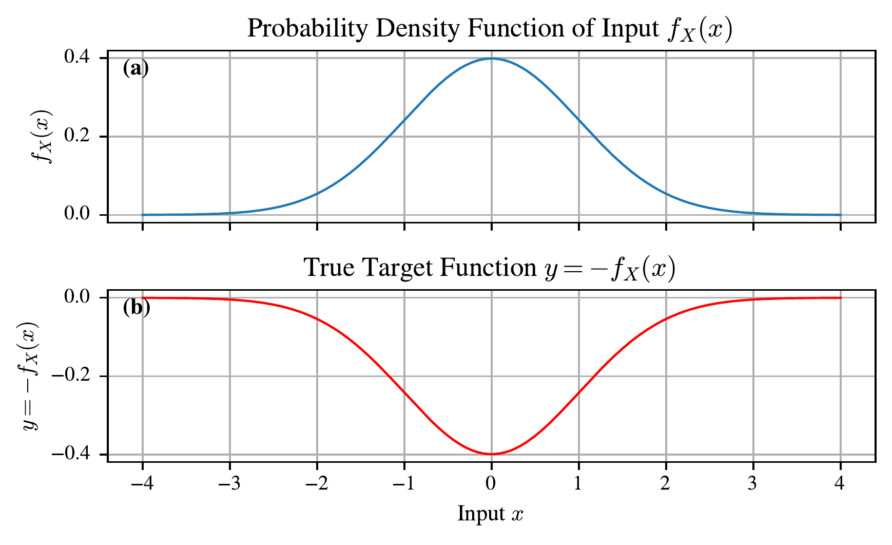
We consider a parsimonious example of where this ReLU neural network linear extrapolation behaviour could be pathological. We assume the true function is an inverted Gaussian, \[\begin{equation} y = - \mathcal{N}\left(0, 1\right)\left(x\right), \end{equation}\](5.3) where \(y\) is the target scalar variable and \(x\) is the input scalar variable. The mean of the normal distribution is 0, and its standard deviation is one for simplicity. We further assume that the probability density function, \(f_X\), of the random variable that generates observations of the inputs, \(X\), is also normally distributed with the same Gaussian, \[\begin{equation} f_X\left(x\right) = \mathcal{N}\left(0, 1\right)\left(x\right), \end{equation}\](5.4) corresponding to most events happening in the central bowl of the negative Gaussian (see Figure 5.2). There is no hard boundary to the support, but the probability of sampling inputs far from the mean becomes vanishingly small. This might be just like natural hazards, where the vast majority of the events are small, but there is some chance that we observe very extreme events. And indeed, we take the existence of a finite upper bound as analogous to our concept of the potential height of tropical cyclone storm surges from Chapters 3 and 4.
We then train a set of 5 simple fully connected ReLU neural networks. Each is trained on a different randomly generated set of 1000 samples. They each have two hidden layers, 32 neurons per hidden layer, and use the Adam optimizer with a learning rate of 0.001 and a batch size of 32 for 100 epochs. These values were not specially selected, and we expect equivalent results for similar ReLU networks.
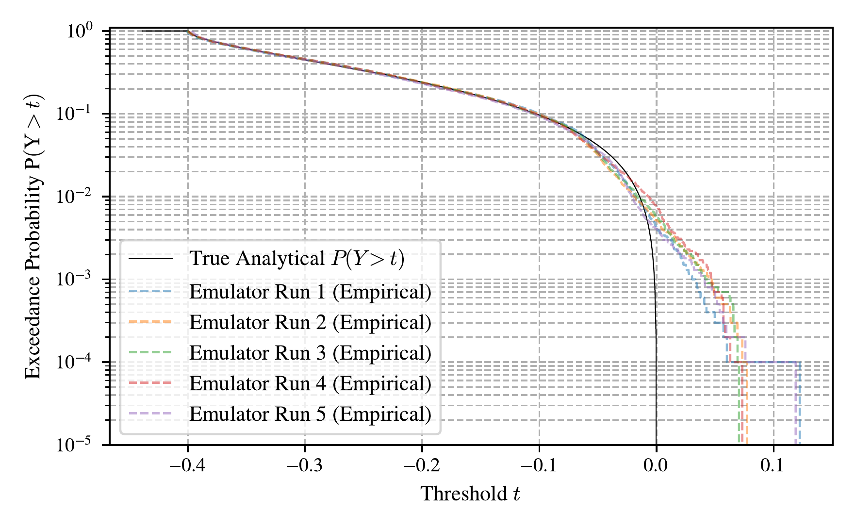
Based on this we can then explore what their exceedance probability curves look like compared to the ground truth (Figure 5.3). In this case, by construction, the true target values, \(y\), cannot exceed 0, and we plot the true exceedance probability curve as a solid black line. The exceedance probability curve for each neural network is estimated empirically by generating a larger sample of 10,000 points, and then using the formula, \[\begin{equation} \mathbb{P}\left(\hat{Y}>\hat{y}_i\right) = 1 - \hat{F}_Y\left(y\right) = 1 - \frac{r}{R+1}, \end{equation}\](5.5) where \(\hat{Y}\) is the random variable corresponding to the neural network’s prediction, \(\hat{y}_i\) is the \(i\)-th largest predicted value, \(r\) is the rank of \(\hat{y}_i\) in the sorted list of predictions, and \(R\) is the total number of predictions. This is a standard way to estimate exceedance probabilities from empirical data (Coles 2001).
We see that all five ReLU neural networks extrapolate incorrectly, predicting that the target variable can exceed 0 (Figure 5.3). This is expected as while all of the networks “see” that the target variable is levelling off, they still experience a positive gradient at the edge of the support, and so extrapolate as a tangent to the true function at that point. This naturally leads to an overestimation of the exceedance probability at high values of the target variable.
While highly simplified, this example highlights that good model performance on average could hide poor performance for the extremes. For natural hazards, extreme performance is everything, and so we must carefully consider the inductive biases we have encoded into our model. In reality, the inputs and outputs are high-dimensional spatial fields evolving over time on a graph (Xu et al. 2020), so it is unclear whether this pathological extrapolation persists in practice, and we must think of ways to test it. We note that bounded activation functions such as tanh or sigmoid saturate naturally and do not exhibit the same unbounded linear extrapolation, which partly motivates the use of tanh after message-passing layers in the SWE-GNN processor (Section Section 5.3.2).
5.3 Model Architecture
In this section, we define the varied neural network architectures evaluated in this study, ranging from simple Multi-Layer Perceptron (MLP) baselines to complex, physics-inspired Graph Neural Networks (GNNs). We describe the architectures first before we describe the data in the next section (Section Section 5.5) in order to motivate the data transformation steps we carry out there. We adopt a consistent notation where the physical domain is represented as a graph, \(\mathcal{G} = \left(\mathcal{V}, \mathcal{E}\right)\), consisting of a set of nodes, \(\mathcal{V}\), and edges, \(\mathcal{E}\).
For each node, \(i \in \mathcal{V}\), the input feature vector, \(\mathbf{x}_i \in \mathbb{R}^{F_{in}}\), where \(F_{in}\) is the number of input features per node, is constructed by concatenating the static topological features, \(\mathbf{x}^{(s)}_i\) (e.g., topography, area), and the dynamic state features from previous time steps, \(\mathbf{x}^{(d)}_i\) (e.g., water levels, velocities). The learning objective for all models is to predict the state increment, \(\hat{\mathbf{y}}_i\), for the next time step (e.g., \(\Delta h, \Delta u, \Delta v\)).
5.3.1 Baseline Models
To rigorously assess the value of graph-based and physics-informed components, we implement four baseline models of increasing complexity.
5.3.1.1 Pointwise-MLP
The simplest baseline is a Pointwise Multi-Layer Perceptron (MLP). This model treats each mesh node, \(i\), as an independent sample, ignoring the graph structure entirely. It approximates the state update function, \(\Phi_{pw}\), which maps the local features of a single node directly to its state increment, \[\begin{equation} \hat{\mathbf{y}}_i = \Phi_{pw}\left(\mathbf{x}_i\right). \end{equation}\](5.6) This baseline tests how much of the fluid dynamics can be inferred purely from local history and static properties without knowledge of neighbouring states.
5.3.1.2 WholeMesh-MLP
The WholeMesh-MLP treats the entire computational domain as a single flat vector. If the mesh contains \(N\) nodes, the input is a flattened vector, \(\mathbf{X} \in \mathbb{R}^{N \cdot F_{in}}\), containing features from all nodes. The model learns a global mapping, \(\Phi_{\text{whole}}\), \[\begin{equation} \hat{\mathbf{Y}} = \Phi_{\text{whole}}\left(\mathbf{X}\right), \end{equation}\](5.7) where \(\hat{\mathbf{Y}} \in \mathbb{R}^{N \cdot F_{\text{out}}}\) is the flattened output vector. While this allows the model to theoretically learn global correlations, it is not permutation invariant, cannot generalise to different mesh sizes, and has a parameter count that scales quadratically with \(N\). It perhaps has the worst physical inductive bias of all the models considered here.
5.3.1.3 Graph Convolutional Network (GCN)
The Graph Convolutional Network (GCN, Kipf 2016) is based on the spectral graph convolution approximation. It incorporates the graph structure, \(\mathcal{E}\), via the adjacency matrix, \(\mathbf{A}\), but assumes isotropic interactions. We employ a single convolutional layer (\(K=1\)) to mimic a first-order numerical flux calculation. In the GCN baseline, this graph convolution layer replaces the physically motivated processor of the SWE-GNN (Section Section 5.3.2), while sharing the same encoder and decoder structure. The latent representation, \(\mathbf{h}_i\), is computed as a degree-normalised weighted average over connected neighbours,
\[\begin{equation} \mathbf{h}_i = \sigma \left( \sum_{j \in \mathcal{N}_i \cup \{i\}} \frac{1}{\sqrt{\tilde{d}_i \tilde{d}_j}} \mathbf{\Theta} \mathbf{x}_j \right), \end{equation}\](5.8) where the sum is over all neighbours \(j\) of node \(i\) plus the node itself, \(\tilde{d}_i\) is the degree (number of connections) of node \(i\) in the self-looped graph, \(\mathbf{\Theta}\) is a learnable weight matrix applied as a linear transformation to the feature vector of each node \(j\), and \(\sigma\) is a non-linear activation function. This is followed by an MLP decoder, \(\hat{\mathbf{y}}_i = \Phi_{\text{dec}}(\mathbf{h}_i)\). The GCN assumes that information transfer is governed solely by connectivity density, ignoring physical edge attributes like distance or orientation.
5.3.1.4 Graph Attention Network (GAT)
The Graph Attention Network (GAT, Veličković et al. 2017) improves upon the GCN by learning anisotropic edge weights. Instead of fixed degree-based normalization, it computes a learnable attention coefficient, \(e_{ij}\), for each edge, \[\begin{equation} e_{ij} = \text{LeakyReLU}\left( \mathbf{a}^T \left[ \mathbf{W}\mathbf{x}_i \parallel \mathbf{W}\mathbf{x}_j \right] \right), \end{equation}\](5.9) where \(\mathbf{W}\mathbf{x}_i\) and \(\mathbf{W}\mathbf{x}_j\) are linear transformations of the node feature vectors, \(\parallel\) denotes their concatenation, and \(\mathbf{a}^T[\cdot]\) is a dot product with a learnable attention vector (equivalently a single linear layer). These coefficients are normalized via softmax to obtain attention weights, \(\alpha_{ij}\). The latent update becomes
\[\begin{equation} \mathbf{h}_i = \sigma \left( \sum_{j \in \mathcal{N}_i} \alpha_{ij} \mathbf{W}\mathbf{x}_j \right). \end{equation}\](5.10) Like the GCN baseline, our GAT implementation uses \(K=1\) layers to maintain a strictly local receptive field analogous to the numerical stencil, but it has the flexibility to “attend” to specific neighbors (e.g., upstream nodes) more than others.
5.3.2 Shallow Water Equation inspired GNN (SWE-GNN)
5.3.2.1 Physical Motivation
The core architecture proposed in this work is the Shallow Water Equation inspired Graph Neural Network (SWE-GNN), originally introduced by Bentivoglio et al. (2023). Unlike the baselines, the SWE-GNN is explicitly designed to emulate the finite volume solution of the Shallow Water Equations (SWEs),
\[\begin{equation} \frac{\partial \mathbf{u}}{\partial t} + \nabla \cdot \mathbf{F}(\mathbf{u}) = \mathbf{s}\left(\mathbf{u}\right), \end{equation}\](5.11) where \(\mathbf{u} = \left[h, q_x, q_y\right]^T\) is the vector of conserved variables (water depth and discharge), \(\mathbf{F}\) represents the fluxes, and \(\mathbf{s}\) represents source terms (bed slope and friction). Because these fluxes are typically computed based on differences between neighbouring triangular elements, the SWE-GNN is structured to mimic this process on the dual graph of the mesh (hence the data transformations we perform in Section Section 5.5).
5.3.2.2 Encoder-Processor-Decoder Structure
The model follows the encoder-processor-decoder paradigm (e.g. Lam et al. 2022), with the message passing function from Bentivoglio et al. (2023).
Encoders: Three separate MLPs encode the input features into latent embeddings: \(\mathbf{h}^{(s)}_i\) for static node features, \(\mathbf{h}^{(d)}_i\) for dynamic state features, and \(\mathbf{h}^{(e)}_{ij}\) for edge attributes (distance and slope).
Processor: The processor performs \(K\) rounds of message passing. In the general message passing framework (Battaglia et al. 2018), each message from a neighbouring source node \(j\) to a destination node \(i\) is an unconstrained learned function of the two node states and any edge attributes (the GCN and GAT baselines in Section Sections 5.3.1.3 and 5.3.1.4 are specific instances). The SWE-GNN constrains this general form so that the update rule is physically motivated. For each edge \(\left(i,j\right)\), an “interaction” vector (analogous to a numerical flux) is computed,
\[\begin{equation} \mathbf{m}_{ij} = \Psi \left(\mathbf{h}^{(s)}_i, \mathbf{h}^{(s)}_j, \mathbf{h}^{(d)}_i, \mathbf{h}^{(d)}_j, \mathbf{h}^{(e)}_{ij} \right) \odot \left( \mathbf{h}^{(d)}_i - \mathbf{h}^{(d)}_j \right), \end{equation}\](5.12) where \(\Psi\) is an MLP that acts as a learned flux coefficient conditioned on the full local state (static, dynamic, and edge features), and \(\odot\) denotes the Hadamard product (element-wise multiplication). The state difference \(\left( \mathbf{h}^{(d)}_i - \mathbf{h}^{(d)}_j \right)\) plays the role of a state gradient driving the flux, ensuring that the message vanishes identically when neighbouring states are equal (as a numerical flux would). This forces the network to learn flux formulations that depend on state differences (analogous to diffusive or advective fluxes). The node state is updated by aggregating these messages, \[\begin{equation} \mathbf{h}^{(d)}_{i} \leftarrow \mathbf{h}^{(d)}_{i} + \sum_{j \in \mathcal{N}_i} \mathbf{m}_{ij}. \end{equation}\](5.13) This process is repeated for \(K\) iterations to allow information to propagate through the graph. After the \(K\) message-passing iterations complete, the GNN activation function is applied once to the final aggregated latent state, \(\mathbf{h}^{(d)}_{i} \leftarrow \sigma\left(\mathbf{h}^{(d)}_{i}\right)\), before decoding. We vary this activation function \(\sigma\left(\cdot\right)\) in our experiments between Tanh (the latent space should saturate, used by Bentivoglio et al. (2023)) and ReLU (as described in Section Section 5.2).
Decoder: A final MLP, \(\Phi_{\text{dec}}\), projects the processed latent state back to physical variables to predict the update, \(\hat{\mathbf{y}}_i = \Phi_{\text{dec}} \left(\mathbf{h}^{(d)}_i\right)\).
The encoders and decoders are implemented as 2-layer MLPs with 128 hidden units and PReLU activations (consistent with Bentivoglio et al. (2023)).
5.4 Evaluation metrics
We evaluate the performance of the models using the root mean square error (RMSE) between the predicted and true peak storm surge heights at each node in the mesh. The RMSE is defined as \[\begin{equation} \mathrm{RMSE} = \sqrt{\frac{1}{N} \sum_{i=1}^{N} \left( \hat{y}_i - y_i \right)^2 }, \end{equation}\](5.14) where \(N\) is the number of samples, \(\hat{y}_i\) is the predicted value, and \(y_i\) is the true value. The lower the value of RMSE the better, with a value of 0 indicating a perfect prediction. The value of RMSE we expect from a simple persistence model depends on the variance of the variables in the dataset. In a scaled dataset a persistence model would have an RMSE of approximately 1. Otherwise we expect the RMSE of a persistence model to be approximately equal to the standard deviation of the target variable.
We also use the Nash-Sutcliffe Efficiency (NSE) to evaluate the models’ performance. The NSE is defined as \[\begin{equation} \mathrm{NSE} = 1 - \frac{\sum_{i=1}^{N} \left( \hat{y}_i - y_i \right)^2 }{\sum_{i=1}^{N} \left( y_i - \bar{y} \right)^2 }, \end{equation}\](5.15) where \(\bar{y}\) is the mean of the true values. The higher the value of NSE the better. The NSE ranges from \(-\infty\) to 1, with a value of 1 indicating a perfect fit, and a value of 0 indicating that the model is no better than using the mean of the true values as a predictor. As our target is the update to the water variables (sea surface height and u and v velocities) at each point, we expect the mean of the true values to be approximately zero. Therefore an NSE of 0 is the expected score for a simple persistence model where nothing changes.
5.5 Data
5.5.1 Data Transformation
For both the training and extreme test datasets Section Sections 5.5.2 and 5.5.3, we process ADCIRC’s netCDF output files to convert them into the dual graph representation required by the SWE-GNN model. Each dual graph node corresponds to the centre of a triangle in the original ADCIRC mesh, and edges connect nodes whose corresponding triangles share an edge. We extract the relevant physical variables at each point for the variables in Table 5.1, and we keep every two hours. Additionally, we calculate ghost cells around the boundary of the domain to properly handle elevation specified boundary conditions during training and inference (although currently we do not use these features). This is described in more detail in Section Section 5.9.
| Symbol | Variable Name ADCIRC | Variable Name SWE-GNN | Units |
|---|---|---|---|
| \(u\) | u-vel |
VX | m s\(^{-1}\) |
| \(v\) | v-vel |
VY | m s\(^{-1}\) |
| \(\eta\) | zeta |
SSH | m |
| \(p\) | pressure |
P | m |
| \(u_{10}\) | windx |
WX | m s\(^{-1}\) |
| \(v_{10}\) | windy |
WY | m s\(^{-1}\) |
5.5.2 Training Data
In the Simon D. A. Thomas (2025c) training dataset we use all of the historical IBTrACS storms from the satellite era (1980-2024) that made landfall in the North Atlantic basin, simulated on the medium-resolution EC95d mesh for the US East Coast (Figure 5.5), as described below.
For the forcing data we use IBTrACS (via NWS=20, Knapp et al. (2018)) that we introduce in Chapter 2 instead of ERA5 (via NWS=13, Hersbach et al. (2020)) in order to avoid some of the well known biases in ERA5 for tropical cyclones, that would lead to relatively underpowered storms compared to IBTrACS, especially for major hurricanes above category 3 (Hodges et al. 2017; Xu et al. 2024). The nominal resolution of ERA5 is 0.25\(^{\circ}\) (approximately 31 km at the equator), but the model continues to be underpowered at resolutions until 1\(^{\circ}\), which can have a significant impact on the representation of tropical cyclones (McTaggart-Cowan et al. 2024; Roberts et al. 2020). It was used as the training data for the GraphCast, GenCast, and NeuralGCM models (Lam et al. 2022; Price et al. 2023; Kochkov et al. 2024). In ERA5 there is little difference in the peak windspeed between a Category 1 to Category 5 tropical cyclone (Xu et al. 2024). This could help to explain why e.g. the GraphCast and GenCast models underpredict the intensity of tropical cyclones and are less skillful than HRES4, despite getting more accurate results for the TC track (Lam et al. 2022; Price et al. 2023).
We take all of the tropical storms that are in the 1980-2024 IBTrACS dataset from the North Atlantic basin that are marked as at some point making landfall (with any part of land in the domain), whose tracks are shown in Figure 5.4. Figure 5.4 shows the tracks of the 228 unique tropical cyclones (TCs) in the dataset, overlaid on the ADCIRC triangular mesh used for the simulations in blue which is the same used in Chapters 3 and 4. The mesh extends from approximately 5\(^{\circ}\)N to 45\(^{\circ}\)N, and from approximately 100\(^{\circ}\)W to 10\(^{\circ}\)W, covering the entire North Atlantic basin and Gulf of Mexico. In Figure 5.5 we see the medium resolution mesh for the US east coast, simulated by ADCIRC, which also includes the Caribbean and Central America. The coastal nodes of the mainland are type 0 normal flow boundary nodes, and the coastal nodes of islands (including barrier islands) are marked in green. The tides can be imposed along the eastern boundary through the blue nodes, whose elevation can be specified to match tidal components.
In Chapters 3 and 4 we used
the NWS=13 meteorological input setting for arbitrary gridded netcdf
inputs to ADCIRC, but here we instead use the NWS=20 ADCIRC
meteorological input setting for the generalised asymmetric Holland wind
model (GAHM). Instead of taking the input as a gridded netcdf of
windspeed and pressure, this takes the data as a tabular input. The
input fields include the location of the centre of the TC at that
timestep, the radius of maximum wind and the velocity of maximum wind,
the outer pressure level and the central pressure level, as well as
additional parameters defining different radii in different quadrants.
The aswip utility uses these multiple radii in different
quadrants to fit different Holland parametric model parameters for each
quadrant. This allows us to incorporate the full asymmetric wind
information recorded in IBTrACS, and most accurately simulate the
available historical storms, but also makes the full input files quite
small and easy to share.
We generate the fort.15 namelist of the ADCIRC forcing
using ADCIRCpy so that the simulations are the same length
as the TC record for each storm. All of the other parameters are kept
the same as in Chapters 3 and 4. We
impose linear meteorological ramping period of one day at the start of
the record to avoid shocks. We use a timestep of 5 seconds, that we find
is more than sufficient for numerical stability on the chosen mesh,
which with a critical Courant number of 0.7 would allow a timestep of 35
seconds. Tides are excluded which corresponds to the open boundary on
the eastern edge of the domain being kept at a fixed elevation of 0.
This training dataset of 228 TCs may seem relatively small, but it is significantly larger than the 100 simulations used to train the original SWE-GNN (Bentivoglio et al. 2023), and the 48 simulations used to train the mSWE-GNN (Bentivoglio et al. 2025). Furthermore, we must be able to test that the ML emulation strategy used can extrapolate to more extreme events than it has seen in the limited record; if it has only seen 40 years’ worth of data, it must be able to predict events more extreme than a 1-in-40-year event, or the emulation technique will have no value for extending risk estimates beyond what can be simulated by standard numerical models. In order to split the data into training, validation, and test sets, we split the data by storms, so that all timesteps from a given storm are only in one of the training, validation, or test sets. To ensure that we can plot Hurricane Katrina (2005) in our results, we place it in the test set. Otherwise we choose 70% (158 storms) for training, 10% (23 storms) for validation, and 20% (47 storms) for testing. We do not vary the split between different runs, and store the data split in a set of configuration yaml files so that we can fairly compare different models on the same data.
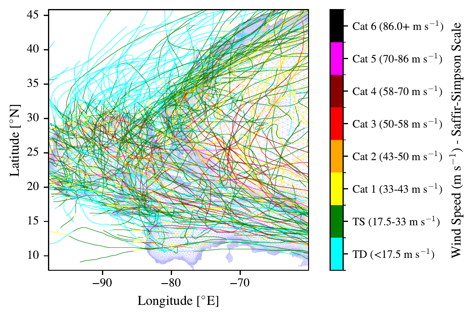
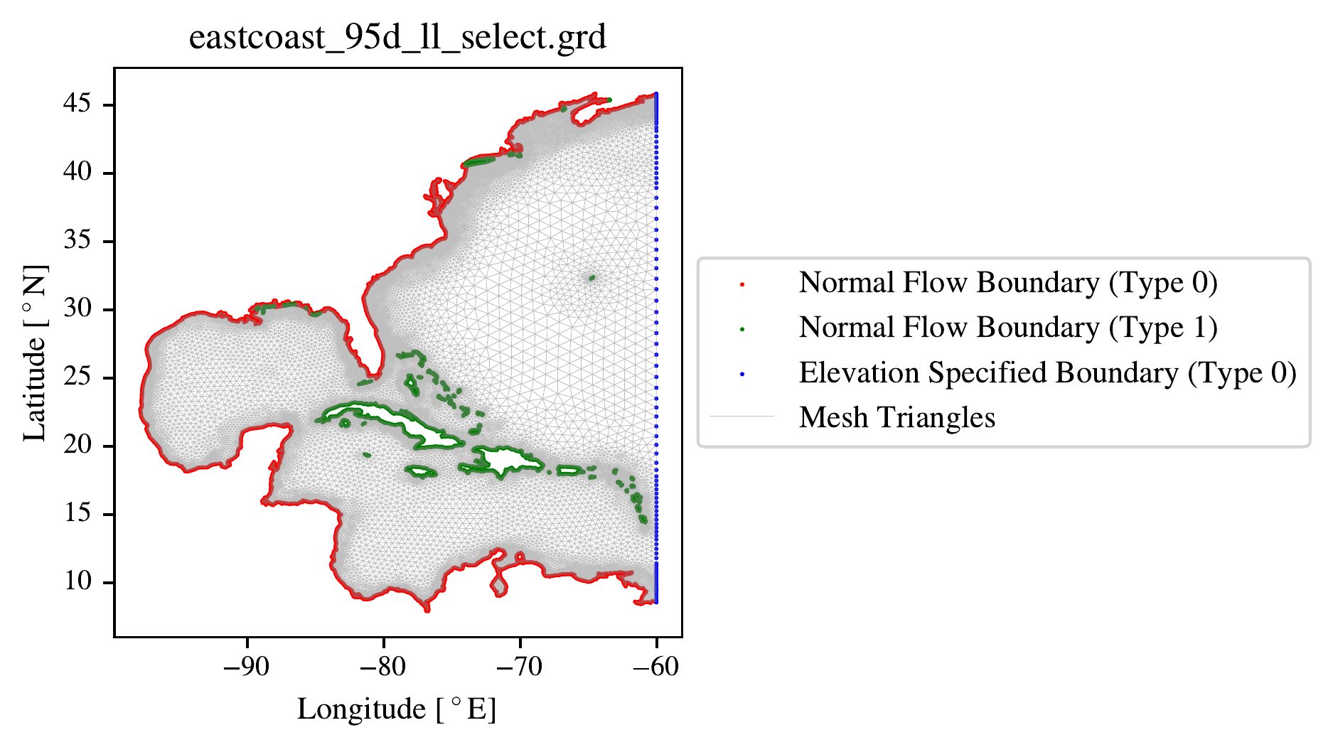
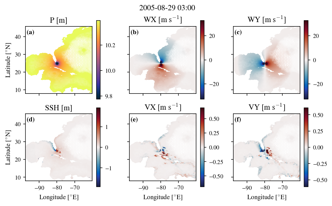
Figure 5.6 shows an example frame from the Hurricane Katrina (2005) ADCIRC simulation, as it moves through the centre of the Gulf of Mexico before turning north. Panels (a-c) show the forcing data: sea surface height (m), 10 m wind speed in the x direction (m s\(^{-1}\)), and 10 m wind speed in the y direction (m s\(^{-1}\)). Panels (d-f) show the corresponding ADCIRC outputs for sea surface height (m), depth-averaged velocity in the x direction (m s\(^{-1}\)), and depth-averaged velocity in the y direction (m s\(^{-1}\)). As we allow storms to be asymmetric in the NWS=20 input the storm’s wind input WX and WY are not orientated as N/S and E/W dipoles respectively, but instead are tilted slightly, which is a change from the idealized inputs for the potential height simulations (Chapters 3 and 4). We can see in panel (d) the small SSH bulge at the centre of the storm, as well as the small positive SSH on the west side of the Florida peninsula. Some currents have been stirred up in panels (e) and (f) as a result of the storm’s previous movement over the south of the Florida peninsula.
5.5.3 Extreme Potential Height Test data
In the Simon D. A. Thomas (2025b) extreme PH test dataset we process the data from Chapter 4 into the same dual graph input format with 2 hour timesteps as the training data, so that it can be a useful extreme test set. There are three different potential height repeats for each of the chosen locations (Galveston, New Orleans, and Miami), for both of the chosen climates (August 2015 and August 2100 in SSP5-8.5 from CESM2 as in Chapter 4), leading to a total of 18 netcdf files in this extreme test set. Each simulation is 7 days long, with one day of meteorological forcing linear ramp up at the start. As highlighted in Chapter 4 the trajectories of the worst-case storms are substantially similar between 2015 and 2100, but with larger and more intense storms in 2100 due to climate change. The repeats for each location are also similar, but with variations in the optimal trajectory angle and translation speed. The largest difference is between the different locations, with New Orleans having the largest absolute storm surge heights due to the large area of shallow water beside it available to pile up a surge, and Miami having the smallest due to its relatively steep bathymetry.
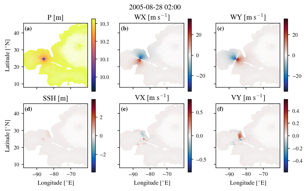
The worst-case storm for Miami in August 2015 is shown in Figure 5.7, with panels (a-c) showing the forcing variables (sea surface pressure, P, 10 m wind speed in the x direction, WX, and 10 m wind speed in the y direction, WY), and panels (d-f) showing the corresponding ADCIRC outputs (sea surface height, SSH, depth-averaged velocity in the x direction, VX, and depth-averaged velocity in the y direction, VY). We show the hurricane as it makes landfall near Miami. In Figure 5.7 there is a strong positive surge along the west and south of the Florida peninsula, and a negative surge to the east of the peninsula, due to the counter-clockwise wind field pushing water away from the east coast. Strong positive surges have also built up against the Bahamas. Very strong currents have built up in areas of shallower water, such as the southwards current and the strong northwards currents that have built up in the Bahamas, corresponding to the water being pushed up against the islands by the TC’s expansive and powerful wind field.
5.6 Results
5.6.1 Model setup
We make some changes to the original SWE-GNN architecture of Bentivoglio et al. (2023) to better suit our application. The full list of input and output features is given in Table 5.3. While Bentivoglio et al. (2023) predicted two variables (water height and velocity magnitude) at each node with a learned residual update, we instead predict the delta update to three variables: water depth, depth-averaged velocity in the \(x\) direction, and depth-averaged velocity in the \(y\) direction. We predict the full velocity vector rather than just its magnitude so that the model can distinguish directional flow patterns. Predicting the delta update (the change between consecutive timesteps) rather than the absolute state is important because the total water depth varies far more in our coastal domain (from 0.1 to 4000 m) than it would in an inland flooding situation (from 0 to 10 m), so predicting the small increment helps the model resolve physically meaningful changes. We also feed sea surface height (SSH), calculated as \(\eta - b\) where \(b\) is the bathymetric depth, as an additional derived dynamic input feature. In total the model has \(7\times p_t\) dynamic input features, 5 static input features, and 2 edge features, and predicts 3 output features (\(\Delta\widehat{\text{WD}}\), \(\Delta\widehat{\text{VX}}\), and \(\Delta\widehat{\text{VY}}\)).
There are encoder MLPs for the dynamic node features (\(7\times p_t\)), the static node features (5), and the edge features (2). The decoder MLP decodes to 3 outputs, which are the updates to the output features. For each MLP, there are two hidden layers, each with 128 hidden features, and the PReLU activation function is used for each, which necessitates 1 additional learned parameter for each activation layer. The hyperparameters used for training the SWE-GNN models are shown in Table 5.2, and the input and output features are shown in Table 5.3.
| Hyperparameter | Value |
|---|---|
| Optimizer | AdamW |
| Initial Learning Rate | \(10^{-3}\) |
| Learning Rate Step Size | 20 epochs |
| Learning Rate Decay Factor (Gamma) | 0.5 |
| Batch Size | 4 |
| Number of Message Passing Layers, \(K\) | 3, 6, 9, 12, 15 |
| Number of Epochs | 100 |
| Hidden Features per MLP Layer | 128 |
| Activation Functions in all MLP Layers | PReLU |
| Activation Functions in Processor | Tanh |
| Feature | Description | Units |
|---|---|---|
| Dynamic node features (\(3\times p_t\)) | ||
| WD | Water depth | m |
| VX | Depth-averaged velocity in x direction | m s\(^{-1}\) |
| VY | Depth-averaged velocity in y direction | m s\(^{-1}\) |
| Features from forcing data (\(3\times p_t\)) | ||
| P | Atmospheric pressure | m |
| WX | 10 m wind velocity in x direction | m s\(^{-1}\) |
| WY | 10 m wind velocity in y direction | m s\(^{-1}\) |
| Derived dynamic node features (\(1\times p_t\)) | ||
| SSH | Sea surface height | m |
| Static node features (5) | ||
| \(b\) | Topography (always negative) | m |
| \(b_x\) | Topography gradient in x direction | m \(^\circ{}^{-1}\) |
| \(b_y\) | Topography gradient in y direction | m \(^\circ{}^{-1}\) |
| \(A\) | Area of the dual cell | m\(^2\) |
| \(t_n\) | Node type | 0 or 1 |
| Edge features (2) | ||
| \(l_{ij}\) | Length of edge between nodes \(i\) and \(j\) | m |
| \(g_{ij}\) | Edge slope between nodes \(i\) and \(j\) | m \(^\circ{}^{-1}\) |
| Output features (\(3\)) | ||
| \(\Delta\widehat{\text{WD}}\) | Change in water depth (or SSH) | m |
| \(\Delta\widehat{\text{VX}}\) | Change in depth-averaged velocity in x direction | m s\(^{-1}\) |
| \(\Delta\widehat{\text{VY}}\) | Change in depth-averaged velocity in y direction | m s\(^{-1}\) |
In the following models, we use the naming convention:
P (\(p_t\)): the number of previous timesteps used as dynamic input features.
K (\(K\)): the number of message passing layers in the processor.
H (\(H\)): the number of hidden features per MLP layer. The same number of hidden features is used for all MLP layers (all of the encoders, the processor, the decoder). In these results we keep this fixed at 128.
ReLU: the activation function used after the message passing layers in the processor. If not specified, Tanh is used.
5.6.2 Example one step delta predictions
Figure 5.8 shows a snapshot from Hurricane Katrina just before landfall, comparing the true delta values from ADCIRC to the predicted delta values from the SWE-GNN-K6 model. Panels (a-c) show the forcing variables (P, WX, WY) at this timestep. Panels (d-f) show the ADCIRC state variables (SSH, VX, VY) at the previous timestep. Panels (g-i) show the true delta values from ADCIRC for (g) SSH, (h) VX, and (i) VY. Panels (j-l) show the predicted delta values from the SWE-GNN-K6 model for (j) SSH, (k) VX, and (l) VY. The true delta update for SSH should have been that the SSH is increasing North of the Mississippi delta, and decreasing south of it, and most of this structure is captured in panel (j), although it is significantly weaker. The x-velocity update in panel (k) is much poorer quality, as the x velocity should be decreasing north of the Mississippi delta and increasing south of it, but is uniformly increasing in panel (k). The y-velocity update in panel (l) is a little better, with some of the positive-negative-positive structure seen in panel (i) being captured in panel (l), although again the magnitudes are significantly lower.
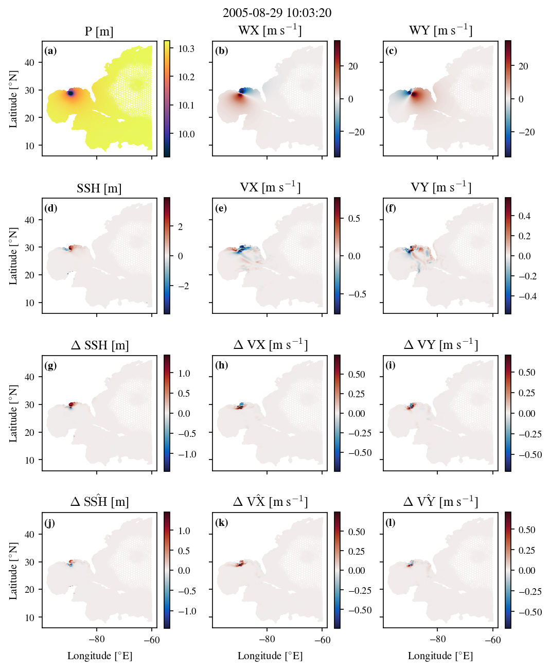
Figure 5.9 shows a snapshot from the extreme test set (Miami 2015 trial 1) comparing the true delta values from ADCIRC to the predicted delta values from the SWE-GNN-K6-P1-H128 model. Panels (a-c) show the forcing variables (P, WX, WY) at this timestep. Panels (d-f) show the ADCIRC state variables (SSH, VX, VY) at the previous timestep. Panels (g-i) show the true delta values from ADCIRC for (g) SSH, (h) VX, and (i) VY. Panels (j-l) show the predicted delta values from the SWE-GNN-K6 model for (j) SSH, (k) VX, and (l) VY. The model is able to capture some of the overall structure of the delta values, but there are significant discrepancies in magnitude and fine details, particularly in the velocity components. The magnitudes of the predicted deltas are generally lower than the true deltas, indicating that the model underestimates the changes in sea surface height and velocity during this extreme event. The worst panel is for SSH in (j) which shows a purely negative update, whereas in reality panel (j) there should be a small area of SSH increase by Miami as the storm makes landfall. In panel (k) the x-velocity update captures some of the positive/negative structure at the south of the Florida peninsula seen in panel (i), but includes a small negative update area within the area that should be the most strongly positive.

5.6.3 Quantitative Evaluation
The quantitative evaluation of the models is detailed in Table 5.4 through Table 5.7. Across all metrics, the domain-specific SWE-GNN architecture consistently outperforms standard graph and MLP baselines, particularly in generalizing to unseen test data and extreme physical events.
5.6.3.0.1 RMSE and Error Reduction
ADCIRC uses a wetting and drying scheme in which dry nodes (those above the waterline) carry zero water depth and zero velocity. In our pipeline these nodes are handled at three levels: during message passing, edges connected to nodes whose entire latent state is zero are excluded from flux computation, so dry nodes neither send nor receive messages; during training, an optional loss mask excludes nodes with water depth below \(10^{-6}\) m; and at inference time, predicted water depths below \(10^{-3}\) m are clamped to zero and the corresponding velocities are zeroed. Together, these steps prevent dry nodes from corrupting the learned dynamics while allowing the model to naturally re-wet nodes as the surge propagates inland.
As shown in Table 5.4 (\(\Delta\)SSH) and Table 5.5 (\(\Delta|U|\)), the SWE-GNN models achieve significantly lower error rates than general-purpose architectures. The optimal model for sea surface height, SWE-GNN-K21-P1-H128-ReLU, achieves a Test RMSE of \(1.73~\text{cm}\), representing a reduction of approximately \(40\%\) compared to the GCN (\(2.87~\text{cm}\)) and Pointwise-MLP (\(3.03~\text{cm}\)) baselines. A similar trend is observed in velocity predictions, where the SWE-GNN-K21-P2 model achieves the lowest Test RMSE of \(0.85~\text{cm~s}^{-1}\). The WholeMesh-MLP baseline performs poorest, likely due to its inability to exploit local spatial inductive biases, resulting in errors exceeding \(3.43~\text{cm}\).
5.6.3.0.2 Goodness-of-Fit (NSE)
The Nash-Sutcliffe Efficiency (NSE) scores presented in Table 5.6 and Table 5.7 further highlight the structural superiority of the physics-informed approach. While standard baselines (GCN, GAT) struggle to achieve NSE scores above \(0.12\) on the test set (indicating predictive power barely better than the mean), the SWE-GNN models consistently achieve scores in the \(0.60\)-\(0.68\) range. This disparity confirms that the specialized message-passing mechanism effectively captures the wave propagation dynamics that standard graph convolutions miss.
5.6.3.0.3 Impact of Receptive Field (\(K\)) and Temporal Context (\(p_t\))
There is a distinct positive correlation between the spatial kernel size \(K\) and model performance. As \(K\) increases from \(3\) to \(21\), the Test NSE for SSH improves from \(0.480\) to \(0.679\) (Table 5.6). This suggests that capturing a wider spatial stencil is critical for the shallow water flows. Additionally, referencing Table 5.7, increasing the temporal context from \(p_t=1\) to \(p_t=3\) improves velocity prediction stability on the Extreme PH dataset, boosting the NSE from \(0.111\) to \(0.281\).
5.6.3.0.4 Generalization to Extreme Events
The “Extreme PH” split tests the models on out-of-distribution storms significantly larger than those seen during training. The results are particularly revealing regarding the choice of activation function after the message-passing layers in the SWE-GNN architecture:
Robustness of Tanh after message passing: The standard SWE-GNN models (using tanh activation after message passing) demonstrate remarkable robustness. The SWE-GNN-K15-P3 model achieves the lowest RMSE on this split for both SSH (\(5.52~\text{cm}\)) and velocity (\(3.92~\text{cm~s}^{-1}\)). In NSE terms, as shown in Table 5.6 and Table 5.7, the SWE-GNN-K15-P3 attains positive NSE scores of \(0.403\) and \(0.281\) respectively, indicating that the model retains substantial predictive skill even under extreme conditions well beyond its training distribution.
Instability of ReLU after message passing: Conversely, the ReLU-based variants, despite performing best on the standard Test set, fail catastrophically on the Extreme PH set. As seen in Table 5.4 and Table 5.5, the SWE-GNN-K21-P1-H128-ReLU error spikes to \(18.01~\text{cm}\) and \(55.73~\text{cm~s}^{-1}\) respectively, resulting in strongly negative NSE scores in Tables 5.6 and 5.7.
This behaviour matches our hypothesis set out in Section Section 5.2, that the linear extrapolation of the ReLU activation function can lead to pathological behaviour, including in this case very high one-step prediction errors.
| \(\Delta\)SSH RMSE [cm] | ||||
| Model | Train | Validation | Test | Extreme PH |
| SWE-GNN-K21-P3-H128 | 1.64 | 1.68 | 1.79 | 5.62 |
| SWE-GNN-K21-P2-H128 | 1.62 | 1.66 | 1.74 | 5.81 |
| SWE-GNN-K21-P1-H128 | 1.65 | 1.68 | 1.77 | 6.44 |
| SWE-GNN-K21-P1-H128-ReLU | 1.61 | 1.64 | 1.73 | 18.01 |
| SWE-GNN-K18-P1-H128 | 1.70 | 1.71 | 1.85 | 6.74 |
| SWE-GNN-K15-P3-H128 | 1.67 | 1.69 | 1.86 | 5.52 |
| SWE-GNN-K15-P1-H128 | 1.63 | 1.69 | 1.81 | 6.72 |
| SWE-GNN-K12-P1-H128 | 1.55 | 1.76 | 1.83 | 7.04 |
| SWE-GNN-K9-P1-H128 | 1.65 | 1.84 | 1.99 | 7.21 |
| SWE-GNN-K6-P1-H128 | 1.67 | 1.86 | 2.00 | 7.29 |
| SWE-GNN-K3-P1-H128-ReLU | 1.99 | 2.01 | 2.16 | 7.63 |
| SWE-GNN-K3-P1-H128 | 1.96 | 2.03 | 2.20 | 7.25 |
| GCN-GNN-P1-H128 | 2.93 | 2.67 | 2.87 | 6.94 |
| GAT-GNN-P1-H128 | 2.94 | 2.68 | 2.88 | 6.96 |
| Pointwise-MLP-P1-H128 | 3.08 | 2.74 | 3.03 | 6.80 |
| WholeMesh-MLP-P1-H128 | 3.14 | 3.05 | 3.43 | 29.66 |
| \(\Delta\mid U\mid\) RMSE [cm s\(^{-1}\)] | ||||
| Model | Train | Validation | Test | Extreme PH |
| SWE-GNN-K21-P3-H128 | 0.76 | 0.88 | 0.87 | 3.94 |
| SWE-GNN-K21-P2-H128 | 0.75 | 0.88 | 0.85 | 3.96 |
| SWE-GNN-K21-P1-H128 | 0.81 | 0.93 | 0.93 | 4.35 |
| SWE-GNN-K21-P1-H128-ReLU | 0.78 | 0.94 | 0.91 | 55.73 |
| SWE-GNN-K18-P1-H128 | 0.80 | 0.93 | 0.93 | 4.50 |
| SWE-GNN-K15-P3-H128 | 0.78 | 0.90 | 0.89 | 3.92 |
| SWE-GNN-K15-P1-H128 | 0.79 | 0.93 | 0.93 | 4.68 |
| SWE-GNN-K12-P1-H128 | 0.76 | 0.96 | 0.93 | 4.95 |
| SWE-GNN-K9-P1-H128 | 0.72 | 0.96 | 0.94 | 5.05 |
| SWE-GNN-K6-P1-H128 | 0.82 | 0.98 | 0.97 | 5.17 |
| SWE-GNN-K3-P1-H128-ReLU | 0.96 | 1.02 | 1.01 | 4.94 |
| SWE-GNN-K3-P1-H128 | 0.90 | 1.02 | 1.02 | 5.30 |
| GCN-GNN-P1-H128 | 1.28 | 1.17 | 1.17 | 4.43 |
| GAT-GNN-P1-H128 | 1.26 | 1.15 | 1.16 | 4.52 |
| Pointwise-MLP-P1-H128 | 1.43 | 1.24 | 1.28 | 4.40 |
| WholeMesh-MLP-P1-H128 | 1.53 | 1.50 | 1.59 | 17.88 |
| \(\Delta\)SSH NSE | ||||
| Model | Train | Validation | Test | Extreme PH |
| SWE-GNN-K21-P3-H128 | 0.731 | 0.639 | 0.664 | 0.395 |
| SWE-GNN-K21-P2-H128 | 0.735 | 0.643 | 0.679 | 0.346 |
| SWE-GNN-K21-P1-H128 | 0.721 | 0.628 | 0.664 | 0.188 |
| SWE-GNN-K21-P1-H128-ReLU | 0.734 | 0.644 | 0.679 | -5.349 |
| SWE-GNN-K18-P1-H128 | 0.704 | 0.616 | 0.635 | 0.111 |
| SWE-GNN-K15-P3-H128 | 0.722 | 0.635 | 0.637 | 0.416 |
| SWE-GNN-K15-P1-H128 | 0.729 | 0.623 | 0.649 | 0.117 |
| SWE-GNN-K12-P1-H128 | 0.753 | 0.593 | 0.640 | 0.029 |
| SWE-GNN-K9-P1-H128 | 0.722 | 0.555 | 0.576 | -0.016 |
| SWE-GNN-K6-P1-H128 | 0.716 | 0.543 | 0.572 | -0.039 |
| SWE-GNN-K3-P1-H128-ReLU | 0.594 | 0.467 | 0.499 | -0.139 |
| SWE-GNN-K3-P1-H128 | 0.608 | 0.455 | 0.480 | -0.029 |
| GCN-GNN-P1-H128 | 0.118 | 0.064 | 0.117 | 0.057 |
| GAT-GNN-P1-H128 | 0.114 | 0.056 | 0.114 | 0.051 |
| Pointwise-MLP-P1-H128 | 0.027 | 0.011 | 0.019 | 0.095 |
| WholeMesh-MLP-P1-H128 | -0.010 | -0.226 | -0.262 | -16.211 |
| \(\Delta\mid U\mid\) NSE | ||||
| Model | Train | Validation | Test | Extreme PH |
| SWE-GNN-K21-P3-H128 | 0.760 | 0.545 | 0.599 | 0.281 |
| SWE-GNN-K21-P2-H128 | 0.761 | 0.536 | 0.607 | 0.270 |
| SWE-GNN-K21-P1-H128 | 0.719 | 0.482 | 0.531 | 0.111 |
| SWE-GNN-K21-P1-H128-ReLU | 0.739 | 0.474 | 0.550 | -144.710 |
| SWE-GNN-K18-P1-H128 | 0.725 | 0.480 | 0.525 | 0.052 |
| SWE-GNN-K15-P3-H128 | 0.746 | 0.528 | 0.580 | 0.291 |
| SWE-GNN-K15-P1-H128 | 0.735 | 0.477 | 0.532 | -0.025 |
| SWE-GNN-K12-P1-H128 | 0.755 | 0.448 | 0.525 | -0.149 |
| SWE-GNN-K9-P1-H128 | 0.775 | 0.447 | 0.518 | -0.198 |
| SWE-GNN-K6-P1-H128 | 0.713 | 0.418 | 0.489 | -0.254 |
| SWE-GNN-K3-P1-H128-ReLU | 0.608 | 0.380 | 0.438 | -0.144 |
| SWE-GNN-K3-P1-H128 | 0.652 | 0.374 | 0.430 | -0.318 |
| GCN-GNN-P1-H128 | 0.301 | 0.183 | 0.248 | 0.079 |
| GAT-GNN-P1-H128 | 0.322 | 0.205 | 0.262 | 0.043 |
| Pointwise-MLP-P1-H128 | 0.121 | 0.079 | 0.107 | 0.093 |
| WholeMesh-MLP-P1-H128 | -0.007 | -0.358 | -0.383 | -13.998 |
5.6.4 Autoregressive Rollout Stability
Despite some of these positive results in the one step ahead prediction task, all the models are extremely numerically unstable when rolled out autoregressively for multiple time steps. Section 10 shows a snapshot from the unstable rollout in the Hurricane Katrina prediction for SWE-GNN-K9-H128 after 49 timesteps, showing the saturated fields extending from the coastlines of the domain. The areas of deep sea in Section 10 are not unreasonable even after 49 timesteps, perhaps as the model has learnt that the updates to the depth integrated velocity etc. in these cells tend to be very low.
5.7 Discussion
5.7.1 Key findings
We can train the model with the very limited forcing data available from tropical cyclones that made landfall in the North American Basin in the satellite period, and we make this data available at Simon D. A. Thomas (2025c).
Whilst all of the models that we train are not yet performant enough to stand in for ADCIRC, the more physically informed SWE-GNN architecture with high \(K\) extrapolates better to the extreme test storms (Simon D. A. Thomas 2025b) than the rest of the models trained (WholeMeshMLP, PointwiseMLP, GAT-GNN, GCN-GNN).
However, subtle architectural choices such as using ReLU vs. tanh after the message passing layers have a large impact on the stability and generalization of the models. The ReLU models perform best on the standard test set, but catastrophically on the extreme test set, likely due to numerical instability when extrapolating to extreme physical values. This matches the pathological behaviour we explore in our toy model in Section Section 5.2.
Increasing the temporal input context from \(P=1\) to \(P=3\) also seems to help with generalization to the extreme test set, likely as the model is able to better capture the temporal dynamics of the storm surge.
The performance of the model improves with increasing number of message passing layers, indicating that deeper models are able to better capture the complex dynamics of storm surge, but this comes at the cost of significantly longer training time (5 minutes per epoch for \(K=3\) vs. 50 minutes per epoch for \(K=21\)).
All the models are extremely numerically unstable, and so cannot yet be used beyond a few time steps without diverging. We discuss strategies for addressing this instability, including differentiable multi-step training and curriculum learning over increasing rollout horizons, in Section Section 5.7.2.1.
Both the training dataset of historical storms (Simon D. A. Thomas 2025c, 38 GB), and the test set of Potential Height storms (Simon D. A. Thomas 2025b, 4 GB) are made available for download via Hugging Face, both with a 2 hour timestep, and on the same mesh. They can be used easily with our branch of the
mSWE-GNNcodebase at https://github.com/sdat2/mSWE-GNN/tree/sdat2 (Simon D. A. Thomas 2025a). Examples of training using Jasmin GPUs are provided in weights and biases at https://wandb.ai/sdat2/surgeflexdelta.A single A100 can roll-out the SWE-GNN model for a 7 day simulation in around 13 seconds, which is around \(100\times\) faster than ADCIRC on the same mesh on a 128-CPU node. This is with no significant optimization of the data loading or processing framework, so there is likely further speedup possible for the same architecture. Therefore, if such a model could be made stable and accurate enough, it would be a useful tool for rapid storm surge prediction.
5.7.2 Future Work
5.7.2.1 Stabilization strategies
To address the observed rapid unphysical saturation of the sea surface height (SSH) and velocity fields, particularly within shallow water regimes, the simplest way to attempt to solve this would be to add noise during training. We propose transforming the deterministic solver into a probabilistic denoising framework. In this regime, the dynamic input state \(\mathbf{u}_t\) is perturbed during training by injecting Gaussian noise, \(\tilde{\mathbf{u}}_t = \mathbf{u}_t + \boldsymbol{\epsilon}\), where \(\boldsymbol{\epsilon} \sim \mathcal{N}(\mathbf{0}, \sigma_{\text{inj}}^2 \mathbf{I})\). Rather than minimizing a point-wise Root Mean Squared Error (RMSE), the network architecture is modified to predict the parameters of a heteroscedastic Gaussian distribution, \(\mathcal{N}(\boldsymbol{\mu}_\theta, \boldsymbol{\Sigma}_\theta)\), over the time-step increments. Consequently, the training objective becomes the minimization of the Gaussian Negative Log Likelihood (NLL), \[\begin{equation} \mathcal{L}_{\text{NLL}} = \frac{1}{2N} \sum_{i=1}^{N} \left( \log \left( \boldsymbol{\sigma}^2_{\theta, i}(\tilde{\mathbf{u}}_t) \right) + \frac{(\Delta \mathbf{u}_{\text{gt}, i} - \boldsymbol{\mu}_{\theta, i}(\tilde{\mathbf{u}}_t))^2}{\boldsymbol{\sigma}^2_{\theta, i}(\tilde{\mathbf{u}}_t)} \right), \end{equation}\](5.16) which naturally penalizes exposure bias by learning a spatially adaptive "artificial viscosity" via the variance term \(\boldsymbol{\sigma}^2_\theta\), thereby stabilizing the trajectory when the model encounters numerical instabilities in shallow regions.
Alternatively, we may implement Differentiable Multi-Step (DMS) training, which directly optimizes the solution trajectory over a horizon of \(k\) autoregressive steps. This is a very common addition and is implemented in Bentivoglio et al. (2023; Bentivoglio et al. 2025; Lam et al. 2022). In this formulation, the predicted state at time \(t+1\), denoted as \(\hat{\mathbf{u}}_{t+1} = \mathbf{u}_t + \mathcal{F}_\theta(\mathbf{u}_t)\), is fed recursively back into the model to generate subsequent predictions without ground-truth correction. The objective function is then computed as the discounted sum of errors over the unrolled horizon, \[\begin{equation} \mathcal{L}_{\text{DMS}} = \sum_{\tau=1}^{k} \gamma^{\tau-1} \| \hat{\mathbf{u}}_{t+\tau} - \mathbf{u}_{t+\tau} \|^2_2, \end{equation}\](5.17) where \(\gamma \in (0, 1]\) acts as a temporal discount factor. While this method explicitly penalizes the accumulation of drift that leads to field saturation, it imposes a linear increase in memory complexity, \(\mathcal{O}\left(k\right)\), which may necessitate the use of gradient checkpointing to remain tractable on our current GPU infrastructure.
Of these strategies, systematically extending the rollout horizon during training is the most promising and immediate next step. Lam et al. (2023) demonstrated a curriculum that first trains on single-step predictions, then fine-tunes on progressively longer autoregressive rollouts (1-step, then 2-step, then 3-step, and so on up to 12-step windows), with each stage warm-started from the previous one. Brandstetter et al. (2022) formalise this as the “pushforward trick”, showing that training on the model’s own multi-step predictions rather than on ground-truth inputs is essential for closing the distribution shift between training and inference. Pfaff et al. (2021) similarly find that injecting noise into the training inputs acts as a simple but effective regulariser against error accumulation. We plan to implement such a stepped rollout curriculum as the key next experiment, as this directly targets the instability we observe and can be combined with longer output timesteps (e.g. 1 hour or 30 minutes instead of 2 hours) to give the model smaller per-step updates to learn.
Finally, the most advanced way to improve stability, we consider an extension to a Neural Ordinary Differential Equation (Neural ODE, Chen et al. 2018) framework, which treats the underlying GNN not as a discrete step-predictor, but as a parameterization of the continuous-time derivative, \(\frac{d\mathbf{u}}{dt} = \mathcal{F}_\theta\left(\mathbf{u}, t\right)\). In this paradigm, the state evolution is recovered by integrating this learned vector field using a black-box numerical solver, \[\begin{equation} \hat{\mathbf{u}}(t + \Delta t) = \mathbf{u}(t) + \int_{t}^{t+\Delta t} \mathcal{F}_\theta\left(\mathbf{u}(\tau), t; \mathcal{G}\right) \, d\tau, \end{equation}\](5.18) where the integral is computed via high-order adaptive schemes such as Runge-Kutta (Chen et al. 2018). This approach inherently stabilizes deep architectures by decoupling the learning of physical dynamics from the discretization error, effectively allowing the solver to take smaller sub-steps in regions of high stiffness, such as near boundaries, where fixed-step methods typically saturate or diverge. However, this stability comes at the cost of significant implementation complexity and training time, requiring the use of adjoint sensitivity methods to backpropagate through the ODE solver without prohibitive memory consumption.
5.7.2.2 Changing the training objective to a diffusion model
GenCast (Price et al. 2023, 2025) show that their diffusion model for weather forecasting outperforms their deterministic autoregressive GNN model (GraphCast Lam et al. 2022, 2023) on all metrics, and has naturally stable rollouts. We could adapt such a problem setup, recasting the machine learning task as denoising a Gaussian random field on the nodes to a generative prediction of update to the state parameters, conditioned on the previous ADCIRC state and the input parameters. The downside of this would be the very large increase in computational cost, as the denoiser network has to be run many times (39 times in Price et al. (2025)) to generate a single time step prediction, both in training and inference. It is likely that this would not be worth the cost, as the weather forecasting problem may be naturally more chaotic than the forced storm surge problem, and so the benefits of a diffusion model may be less pronounced here.
5.7.2.3 Improvements to the Graph Neural Network architecture
We can improve the structure by using attributes of the graph that we have already calculated and that were used in Bentivoglio et al. (2025). Standard GNNs struggle with open boundaries where external forcing (e.g., tides) drives the flow. In (Simon D. A. Thomas 2025c, 2025b) we calculate the “ghost nodes” at the domain boundaries. A ghost node \(j\) connected to a boundary node \(i\) holds the prescribed boundary value (e.g., tidal level \(h_{tide}\)) as its feature \(\mathbf{x}^{(d)}_j\). The message passing mechanism \(\mathbf{m}_{ij}\) then automatically computes the flux exchange between the domain and the boundary, allowing the model to handle time-varying external forcing.
Our current pipeline already supplies both water depth WD and sea-surface height \(\text{SSH} = \text{WD} + b\) to the model (the latter derived on the fly from the static bathymetry), so the network has access to both representations. Because we predict deltas (\(\Delta\text{WD} = \Delta\eta\)), the prediction target is identical either way. A minor refinement would be to switch the recurrent accumulator from WD to \(\eta\), so that the state fed back during autoregressive rollout sits on a narrower numerical range rather than carrying a large bathymetric offset; in practice, however, the per-feature scaling already applied to the inputs largely addresses this.
We could also follow the evolution from Bentivoglio et al. (2023) to Bentivoglio et al. (2025) where we implement a multi-scale mesh structure. The Courant-Friedrichs-Lewy (CFL) condition limits the time-step \(\Delta t\) in explicit numerical solvers such as ADCIRC; although the CFL condition does not directly apply to ML models, an analogous constraint exists: in a single message-passing step each node can only receive information from its immediate neighbours, so fast-travelling waves can outrun the receptive field. Stacking \(K > 1\) processor layers addresses this by allowing information to propagate over \(K\) hops in one time-step, effectively expanding the receptive field to \[\begin{equation} \text{RF}\left(\hat{\mathbf{y}}_i\right) = \{ j \mid \text{dist}(i, j) \le K \}, \end{equation}\](5.19) and enabling the network to capture wave propagation speeds that a single-layer model would miss. Beyond stacking layers on a single graph, Bentivoglio et al. (2025) implement a multi-scale mesh structure by coarsening the mesh into a hierarchy of graphs \(\mathcal{G}_0, \mathcal{G}_1, \ldots, \mathcal{G}_L\), where each level \(l\) has its own adjacency matrix \(\mathbf{A}^{(l)}\) and node features \(\mathbf{X}^{(l)}\). During message passing, information is exchanged not only within each scale but also between scales via learned projection operators. GraphCast uses a conceptually similar multi-resolution icosahedral mesh hierarchy (Lam et al. 2022). This multi-scale approach enables the model to capture both local dynamics on fine meshes and global patterns on coarse meshes, improving its ability to model complex wave phenomena across different spatial resolutions, and may also permit stable integration with longer timesteps.
We should also try to compare against all of the state of the art GNN architectures for physical modelling (see e.g., Ma and Tang 2021). At the moment, we only use GAT (Veličković et al. 2017) and GCN (Kipf 2016) as baselines, and even then with \(K=1\) hops, where we can only use information from direct neighbours, and both GAT-GNN and GCN-GNN do not use edge attributes. In order to make a fairer comparison, and better explore whether the SWE-GNN architecture (Bentivoglio et al. 2023) is indeed better suited to the problem, we should implement more recent GNN architectures that use edge attributes and multiple hops (e.g., Taghizadeh et al. 2025).
5.7.2.4 Comparison to other storm surge emulators
Rivera-Casillas et al. (2025) emulate the ADCIRC model driven purely by the tidal potential using their ‘Multiple-Input Temporal Operator Network’ MITONet (based on DeepONet (Lu et al. 2019)), particularly focusing on the Shinnecock Inlet case from ADCIRC’s test suite. They are able to show high accuracy and stability over long rollouts, alongside the ability to learn with multiple friction coefficients. By using a DeepONet architecture, they are able to sidestep the problem of calculating Fourier coefficients on an unstructured grid that would arise if they had used a Fourier neural operator. They reference that OceanNet (Chattopadhyay et al. 2024) was effectively able to use a Fourier neural operator to deal with an ocean forced by wind and pressure. As a combination of GNNs and neural operators, Graph Neural Operators (Li et al. 2020; Li et al. 2025) may have some advantages over more standard GNNs, as they could achieve better generalization to different meshes through zero-shot super-resolution. While standard DeepONets handle unstructured coordinates natively, recent architectures have explicitly hybridized them with Graph Neural Networks to better capture topological connectivity on irregular grids. For example, GraphDeepONet (Cho et al. 2024) utilizes GNNs to improve robustness on irregular time-dependent domains, while GS-PI-DeepONet (Karumuri et al. 2025) integrates graph structures to strictly enforce geometric relationships in unstructured finite element meshes.
5.7.2.5 Possible coastal problems
Furner et al. (2024) use a CNN with a narrow \(3\times3\) filter stencil to emulate the MITgcm ocean model of a highly idealized Southern Ocean with land peninsulas disrupting the circumpolar flow. They find that while the 12 hour delta performance is excellent in most of the domain, the CNN struggles near the coast where it is less skilful than a persistence baseline. We cannot use a CNN here because of the unstructured mesh, and we hope that performing the GNN processing on the dual graph where coastal nodes are only able to exchange information with ocean nodes will help the model learn to respect the coastline boundary conditions better.
5.7.2.6 Improving the training data
It is possible that the 2 hour timestep used by our training and test data (Simon D. A. Thomas 2025c, 2025b) is too long for the model to learn the dynamics accurately. The data output timestep could be reduced to 1 hour or even 30 minutes, which would give the model more data to learn from, and also reduce the size of the updates that the model has to learn to predict. This would come at the cost of increasing the size of the training data significantly, and so would require more storage space and longer training times.
Beyond refining the temporal resolution, more training data could be generated in at least two ways. First, a synthetic tropical cyclone catalogue (produced, for example, by the statistical downscaling approach of Emanuel et al. 2006) could be run through ADCIRC, cheaply multiplying the number of storm events available for training. Second, ADCIRC could be forced continuously with reanalysis for several decades, as Xie et al. (2023) do with the FVCOM hydrodynamic model in the Pearl River Estuary, which avoids relying on a storm catalogue altogether but produces a dataset dominated by low-surge conditions and is computationally expensive.
The graph neural network models should be able to generalise between different ADCIRC meshes, as long as the other ADCIRC model parameters are either kept the same or included as input features. Therefore, we could create training data based on different locations, such as SE Asia (to be consistent with Chapter 2). A more heterogeneous training dataset may help the model learn the underlying physics better, and improve its ability to generalise to unseen storms.
5.7.2.7 Other ways of creating extreme test sets
The extreme test created here (Simon D. A. Thomas 2025b) is based on the Potential Height method of Chapter 4, which creates physically plausible extreme storms. There are no obvious comparisons for extreme storm surge test sets in the literature, but there are other methods for creating extreme test sets for climate and weather models that could be adapted for storm surge modelling.
One method is the rare event algorithm utilized by Ragone et al. (2018). This method employs an iterative “cloning and pruning” strategy to steer the global climate model dynamics towards the tails of the probability distribution. By periodically selecting ensemble members that exhibit higher anomalies and restarting them with slight perturbations, the ensemble naturally drifts towards physically plausible but extremely rare states (such as 1-in-10,000 year heatwaves as in Gessner et al. 2021). This allows for the quantification of events with return periods far exceeding the available simulation time, offering a computational speedup of orders of magnitude compared to standard brute-force integration. This is an alternative way to create extreme meteorological events such as tropical cyclones that could then be used to run the ADCIRC model. This would trade the simplifications made in the potential size derivation in Chapter 2 for the dynamical biases of a climate model, but it would also guarantee the whole forcing field was physically plausible, rather than just a single TC. It would also allow us to generalise to extratropical cyclones and hybrid storms.
5.8 Conclusion
We have created a valuable dataset of storm surge simulations using the ADCIRC model, which is adapted for use with the SWE-GNN architecture (Simon D. A. Thomas 2025c). The potential height simulations from Chapter 4 are used to create a unique extreme test set that allows us to probe how successfully the emulators extrapolate to very extreme unseen conditions (Simon D. A. Thomas 2025b). We train a set of emulators with different architectures and hyperparameters, and find that the SWE-GNN architecture with more message passing steps \(K\) is able to extrapolate better to the extreme test set than the other architectures tested. However, all models are still extremely numerically unstable when rolled out autoregressively for multiple time steps, and so further work is needed to improve the stability of the models during autoregressive rollouts, potentially through techniques such as multistep ahead training losses or incorporating physical constraints into the model architecture. Our published datasets (Simon D. A. Thomas 2025c, 2025b) aim to make the next challenge easier for the field by making the problem ‘data ready’ for future ML attempts.
Open Science
The code for creating the ADCIRC training data and processing it is
available at https://github.com/sdat2/PotentialHeight (Simon Donald Alistair Thomas
2025) which builds on the sithom utility library
(Thomas
2024). The training data is published at Simon D. A. Thomas (2025c)
and the test data at Simon D. A. Thomas (2025b).
The code for training the SWE-GNN models is available at https://github.com/sdat2/mSWE-GNN/tree/sdat2 (Simon D. A.
Thomas 2025a).
5.9 Appendix: Dual graph calculations
To get the training method to work, we do some calculations to transform the data from its original triangular component mesh to its corresponding dual graph.
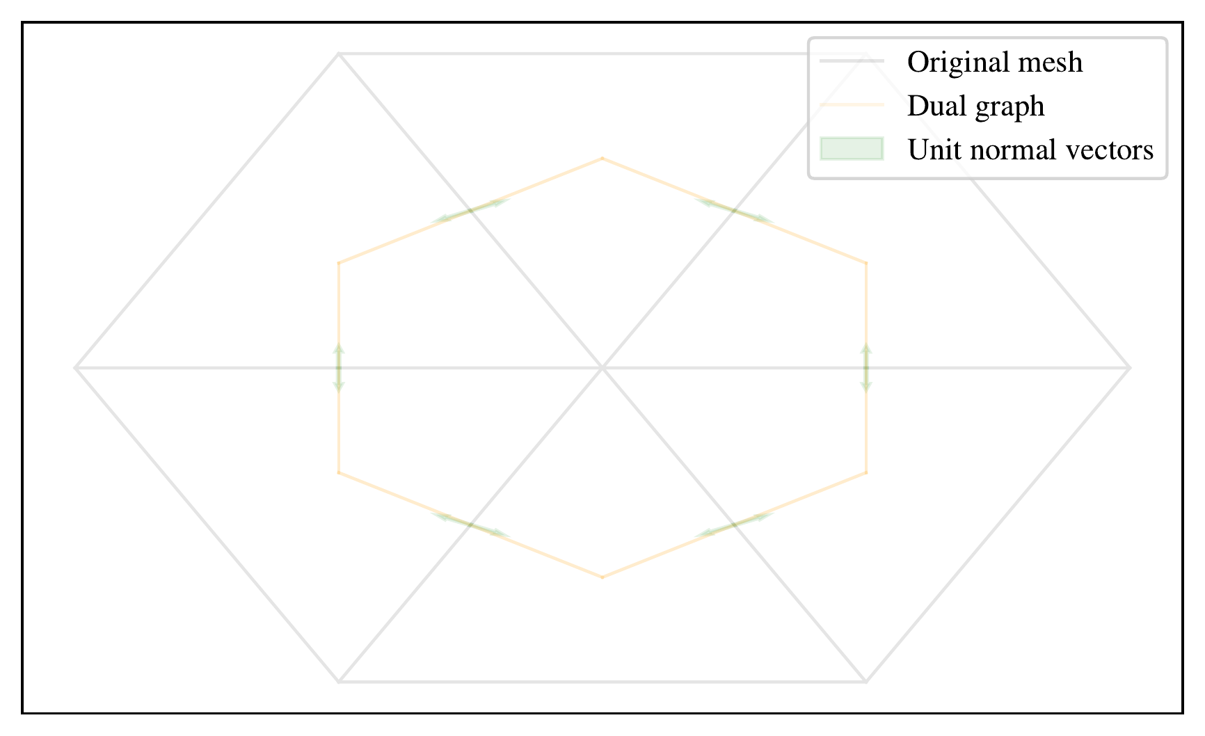
The attributes of each dual graph node is taken as the mean of the three nodes in the triangular element. Therefore, its position is at the centre of the triangular element, as shown in Figure 5.10. Two dual graph nodes \(i\) and \(j\) are adjacent if the triangular elements they are based on share an edge. Each dual graph edge has static properties \(\epsilon_{ij}=\left(\hat{\vec{n}}_{ij}, l_{ij}\right)\). \(\hat{\vec{n}}_{ij}\) is the outward unit normal vector, defined as orthogonal to the triangular mesh edge that joins the two dual graph nodes, and outward in that it points in the same sense as the position vector \(i\) to \(j\). These outward unit normal vectors are shown in green for \(\hat{\vec{n}}_{ij}\) and \(\hat{\vec{n}}_{ji}\) in Figure 5.10.
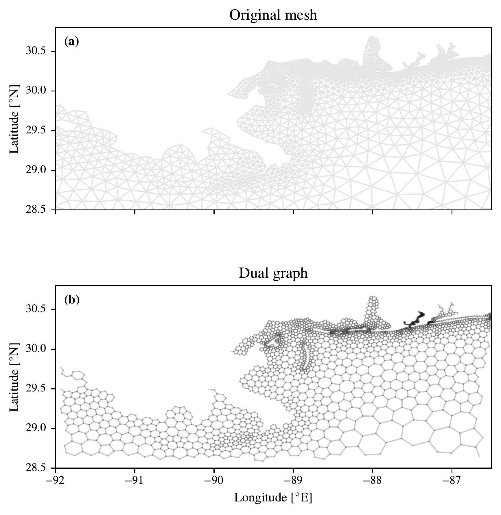
To show what this looks like for the ADCIRC mesh, in Figure 5.11 we show the dual graph transformation for a part of the mesh in the region of New Orleans. As can be seen, the mesh is refined in detail around the barrier islands and near the coast of New Orleans, and this is also present in the dual graph.
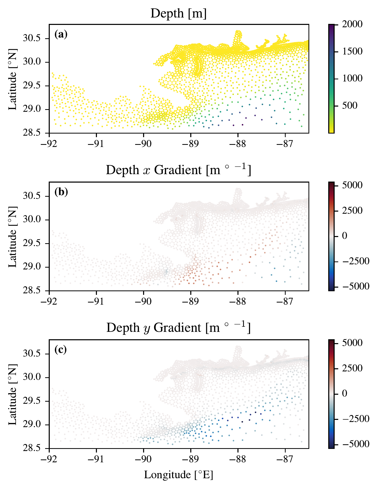
To get a better sense of what the transformation means for the variables on the ADCIRC mesh in Figure 5.12 we show how the depth and its \(x\) and \(y\) gradients appear on the dual graph. In panel (a) we can see that the majority of the New Orleans is shallow (\(<\)100 m), but there is a deeper area to the south east of the plot that is deeper, getting up to 2000 m depth. We can calculate the gradient of each dual graph node for each variable by considering the three points that make up each mesh point \(m\), \(n\), \(o\). The \(x\) and \(y\) coordinates for each mesh point can be used with the variable (in this case \(d\)) to calculate the normal vector to the plane implied by taking the cross product of the edges of two of the sides. From this we can calculate the gradient of the plane that includes the dual graph node in \(x\) and \(y\). As is shown in Figure 5.12 (b-c) the depth increases as you go to the deeper area in the south east leading to a positive \(x\) gradient in this area and the depth decreases as you go further north out of this deep area leading to a negative \(y\) gradient.
References
Which has been succeeded by WeatherBench.v2 (Rasp et al. 2024).↩︎
See my adaptation of their Bentivoglio et al. (2023; Bentivoglio et al. 2025) code at https://github.com/sdat2/mSWE-GNN/tree/sdat2 (Simon D. A. Thomas 2025a).↩︎
An inductive bias is any architectural assumption built into a machine learning model that constrains the hypothesis space and guides generalisation (Battaglia et al. 2018). Every design choice, from weight sharing in CNNs (encoding translation equivariance) to message passing in GNNs (encoding that interactions occur over graph structure), constitutes an inductive bias. A fully connected MLP has minimal inductive bias: it can in principle approximate any function, but equally receives no structural guidance towards the correct one.↩︎
Personal communication from Matthew Wilson at IUGG 2023 and from Ferran Alet 2024-02-14↩︎